Data-Driven Modeling

Data to Dynamics

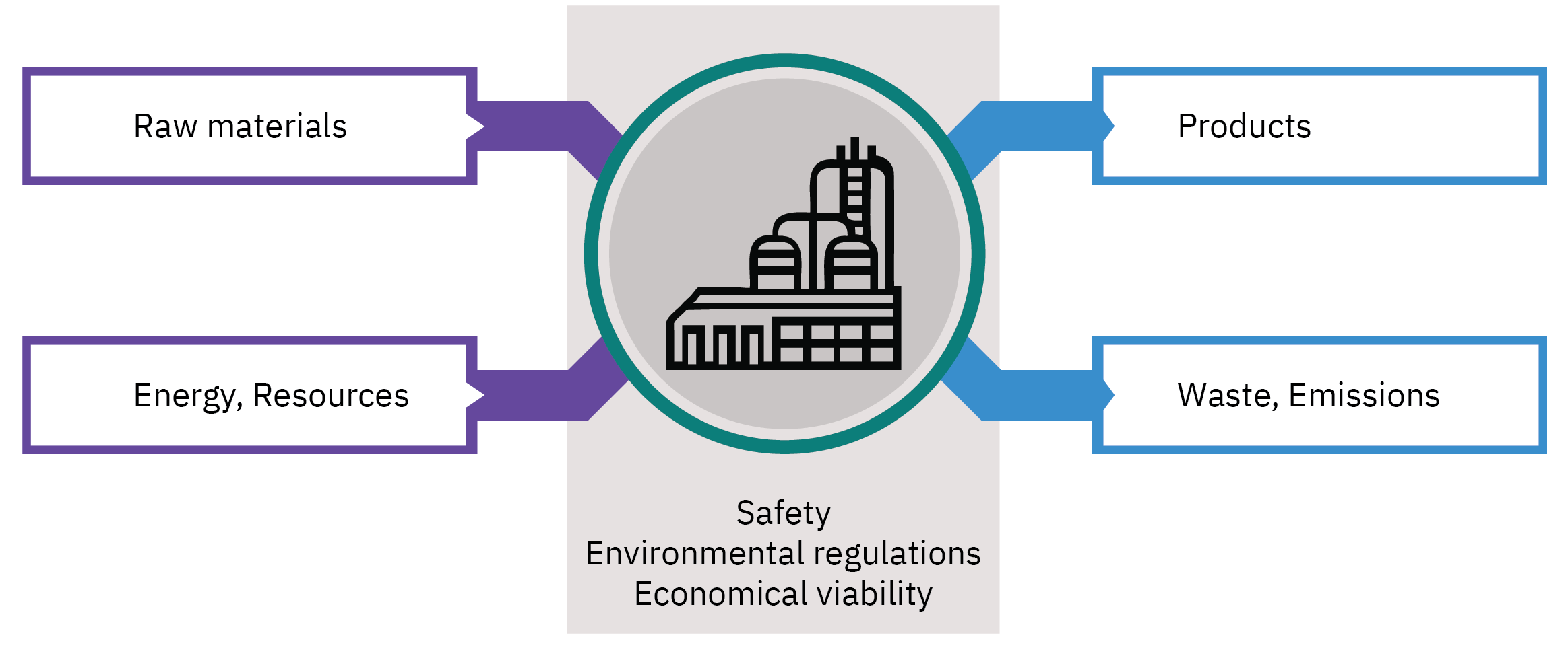
Chemical processes
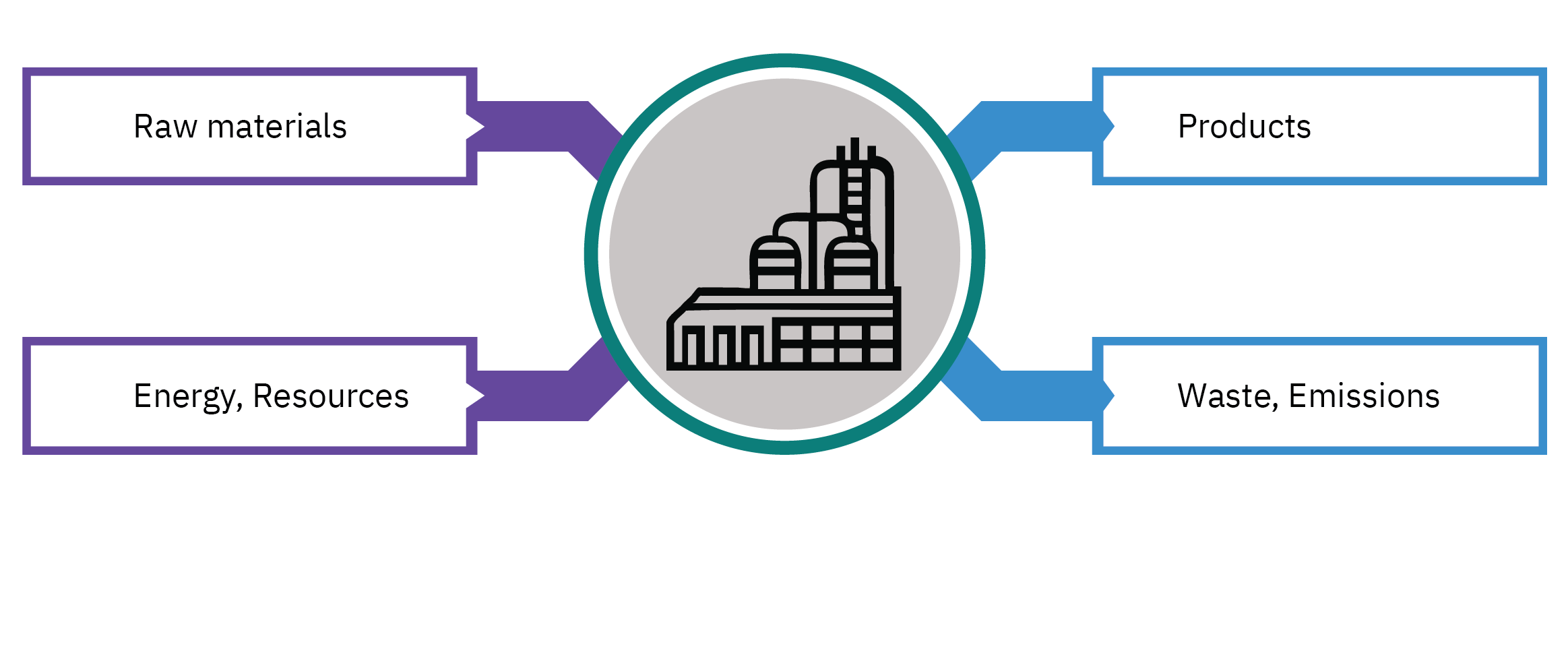
Impact on daily life

  • Food production, water treatment, healthcare, pharmaceuticals
  • Energy, automotive industry, manufacturing
  • \Rightarrow Rely on chemical process industry for ingredients, raw materials, and enabling technologies

Sustainability focus

  • Responsible resource utilization
  • Minimization of environmental impact
  • Long-term viability and competitiveness

Process components

  • Unit operations: mixing, heat exchange, mass transfer, reaction
  • Performed in specific sequence to achieve objectives

Chemical processes

  • Chemical processes are complex systems that transform raw materials into valuable products.
  • Optimal process operations require efficient and effective control
  • Data-driven approaches enable better understanding of process behavior and inform control strategies

Course outline

  1. Nature of chemical processes
  2. Nature of chemical engineering data
  3. Data driven approaches to process characterization and dynamics
  4. Latent variable methods
  5. Nonlinear and machine learning models
  6. Model lifecycle and deployment

About me

Ranjeet Utikar

  • Associate Professor, Chemical Engineering, Curtin University, Australia

  • SMILE Lab (Sustainable Manufacturing and Intelligent Process Engineering)

  • Research interests

    • Sustainable energy and bioprocesses
    • Process modeling and scale-up
    • Process intensification and multiphase flows
  • Experience

    • 100+ peer-reviewed publications
    • Industrial experience: chemical, oil & gas, resources, biotechnology
    • Entrepreneur: Tridiagonal Solutions, Vivira Process Technologies
Objectives and expectations

Learning objectives

At the end of the course you should be able to:

  • Gain an overview of the nature and characteristics of chemical engineering data
  • Understand data-driven approaches to characterize process dynamics
  • Be introduced to latent variable methods for dimensionality reduction
  • Explore nonlinear and machine learning models for chemical processes
  • Learn about model lifecycle from development to deployment

Course philosophy

  • Develop insight into problem-solving (setting up and solving problems independently)
  • Learn to critically assess models and results
  • Ask questions as they arise
  • Knowledge is the key - get maximum value from the course
  • Learn from mistakes, interact, and engage

Your turn

  • Form groups of 4-5 people.

  • Introduce yourself to your group members. Tell them:

    • Who you are?
    • Why you enrolled into this course?

\Rightarrow What are your Objectives and Expectations?

Nature of chemical processes

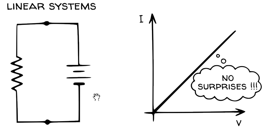
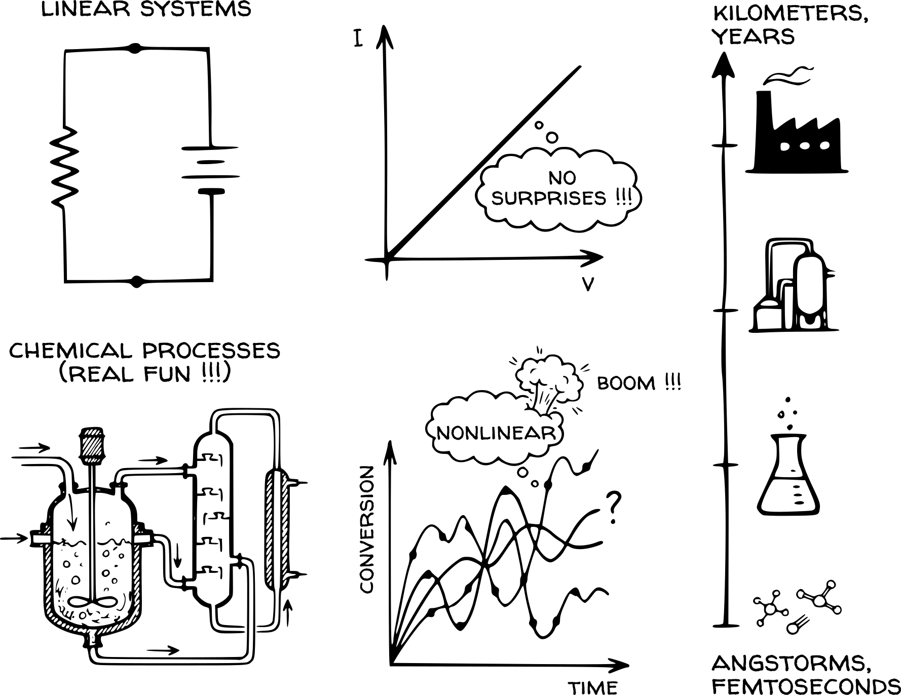
Linear systems

  • Deterministic and predictable
  • Output proportional to input (V = IR, F = kx)
  • Doubled input \Rightarrow doubled response
  • Superposition: effects simply add up
  • Design complex systems with high confidence
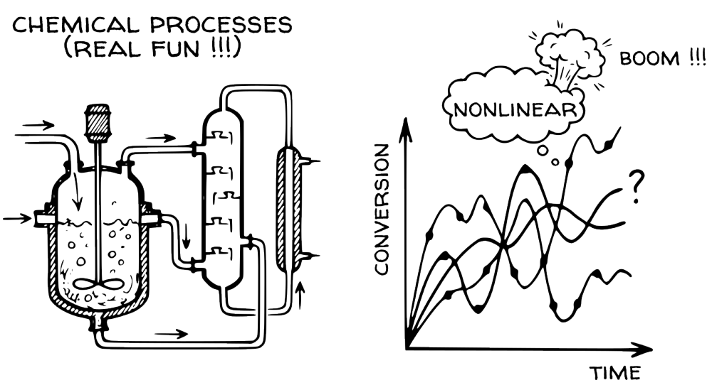
Nonlinear systems

  • Stochastic nature
  • Inherent process complexity
  • Sources of non-linearity
  • Multivariable & Coupled
  • One variable change affects multiple outputs
  • Difficult to isolate variables (e.g., distillation)
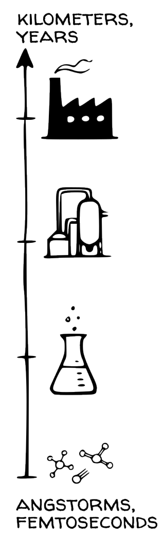
Time and length scales

  • Time-varying behavior
    • Catalyst sintering (~years)
    • Heat exchanger fouling (~months)
    • Ambient temp swings (daily/seasonal)
  • Vast scales involved
    • Molecular (Å, femtoseconds)
    • Unit operations (meters, hours)
    • Plant lifecycle (km, years)

Chemical systems

  • Inherently complex.
  • Non-linear relationships between variables
  • Tight coupling
  • Dynamic behavior that evolves over time
  • Phenomena occurring across multiple scales

\Rightarrow Challenging to design, difficult to predict, hard to control, and complex to optimize
Computational models

Computational models

  • Models enable
    • simulation of process behavior,
    • prediction of responses to disturbances,
    • design of effective control strategies, and
    • optimization of operations
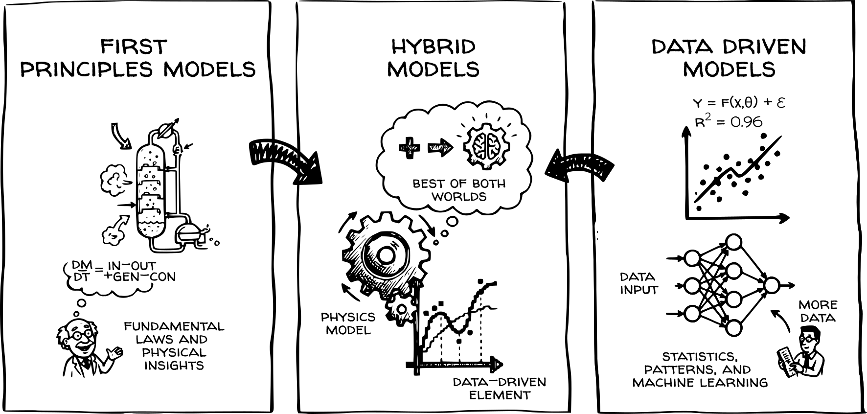
  • Classification
    • Mechanistic or first-principles models
    • Empirical or data-driven models
    • Hybrid approaches

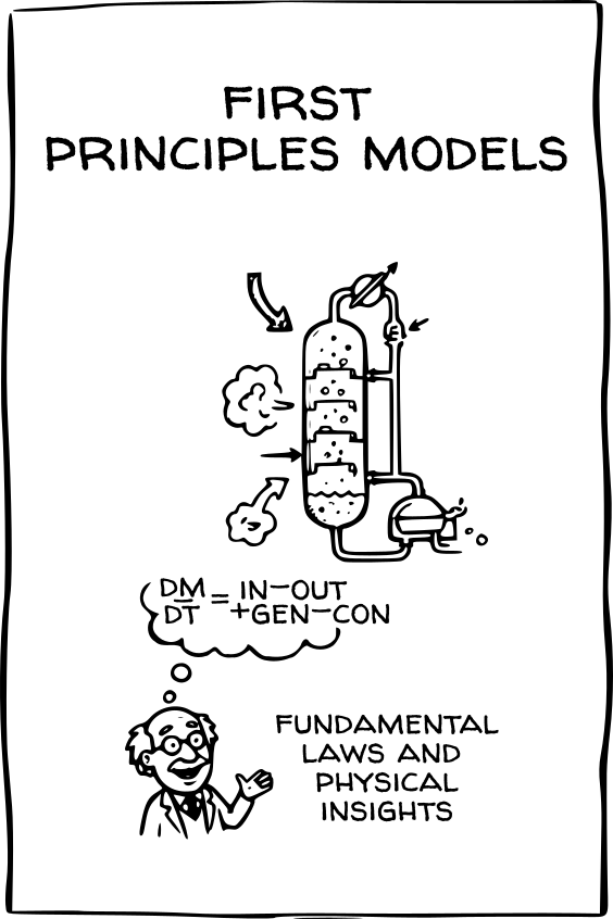
First principles models

  • Formalize conservation laws
    • Mass, energy, momentum
  • Constitutive equations
    • Transport rates, kinetics, thermodynamics
  • Mathematical structure
    • Algebraic, ODEs, or PDEs
  • Physical constraints
    • Enforce limits (e.g., non-negativity)
  • Outcome
    • Encode evolution of process variables

First principles models

Advantages

  • Parameters have physical meaning
  • Process behavior is interpretable
  • Valid outside training range (extrapolatable)

Limitations

  • Difficult to develop (high expertise)
  • Limited understanding of complex mechanisms
  • Computationally expensive to solve
  • Plant-model mismatch common
  • Challenging for online control/optimization

First principles models

  • Essential when data is scarce or expensive
  • Required for process development and scale-up
  • Enables extrapolation beyond historical data
  • Analysis of rare/unsafe events (e.g., runaways)
  • Provides physical bounds for data-driven models

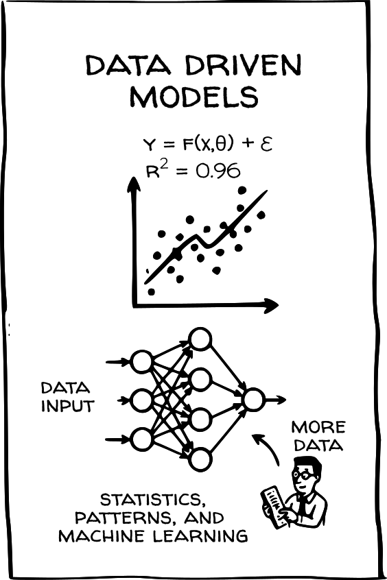
Data-driven models

  • Based on statistical relationships between measured variables
  • Exploits large volumes of operational data (DCS, sensors, historians)
  • Constructs input-output mappings without mechanistic knowledge
  • Effective when:
    • Phenomena are too complex for first principles
    • Mechanisms are poorly understood
    • Rapid development is required

Traditional empirical modeling

  • Statistical regression (Linear, PLS)
    • Captures linear relationships
    • Handles high-dimensional data
  • Time-series models (ARMAX, State-space)
    • Captures temporal dynamics and feedback loops
  • Benefits
    • Computational efficiency
    • Theoretical guarantees (confidence intervals)
    • Interpretability via coefficients

Modern machine learning

  • Learns relationships directly from data (no functional form assumed)
  • Neural Networks: Approximate arbitrary nonlinear relationships
  • Tree-based ensembles (Random Forests, Gradient Boosting):
    • Handle regime transitions
    • Automatic feature selection
  • Support Vector Machines: Classification and nonlinear regression
  • Trade-off: High flexibility vs. limited interpretability

Classification dimensions

  • Static vs. Dynamic
    • Time dependence (differential equations vs. direct mapping)
  • Linear vs. Nonlinear
    • Superposition vs. interactions/thresholds
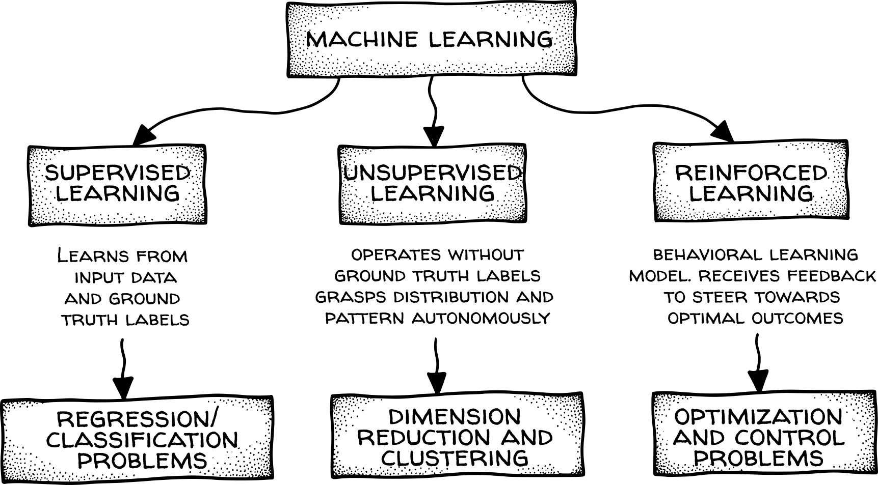
  • Learning Paradigm
    • Supervised (labeled data)
    • Unsupervised (latent structure)
    • Reinforcement (trial and error)
  • Task
    • Regression (continuous) vs. Classification (discrete)
Practical advantages

  • Minimal domain expertise required
  • Rapid model development (minutes/hours vs. weeks/months)
  • Captures complex interactions & nonlinearities naturally
  • Modest computational cost (real-time capable)
  • Reproduces plant behavior with sufficient data

Fundamental limitations

  • Lack physical interpretation (black-box)
  • Unreliable extrapolation beyond training data
  • Susceptible to model degradation (drift/fouling)
  • High data requirements (high dimensionality)
  • Correlation not equal to Causality
  • May violate physical constraints (mass/energy balances)

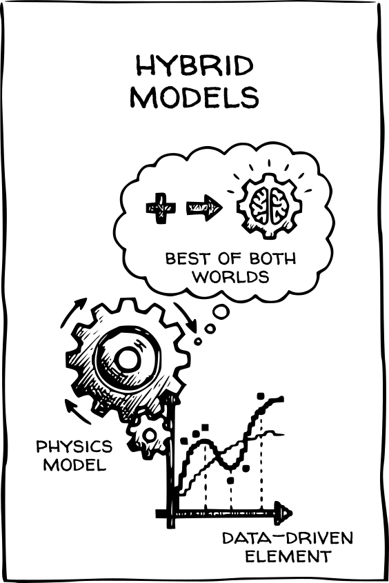
Hybrid models

  • Combine mechanistic and data-driven approaches
  • Structure
    • Physical equations for well-understood parts
    • ML/Stats for difficult-to-model phenomena
  • Benefits
    • Extrapolation capability (via physical backbone)
    • Handles theoretical knowledge gaps (via data)
    • Reduced parameter learning burden

Hybrid models architectures

  • Serial configurations
    • FP model predicts nominal \rightarrow ML corrects residuals
  • Parallel structures
    • Output = Mechanistic term + Empirical term
  • Nested formulations
    • ML embedded in mechanistic eqns (e.g. rate laws)
  • Selection depends on available knowledge and model accuracy

Hybrid models synergistic advantages

  • Lower data requirements (inductive bias)
  • Better extrapolation validity
  • Targeted experimentation
  • Root-cause analysis enablement
  • Balanced computational effort

Hybrid models challenges

  • High expertise demanded (Process + ML)
  • Complex parameter identification
  • Risk of structural bias from FP component
  • Optimization convergence issues
  • Complex maintenance (update FP + recalibrate ML)

Selecting a modeling approach

Criterion First-Principles Data-Driven Hybrid
Process knowledge required High Low Medium
Operational data required Low High Medium
Development time Weeks-months Days-weeks Weeks
Computational cost (training) Low Medium-High High
Computational cost (prediction) High Low Medium
Extrapolation capability High Low Medium-High
Interpretability High Low Medium
Expertise required Process engineering Statistics/ML Both
Maintenance burden Low High Medium
Primary applications Design, scale-up, regulatory Control, monitoring Process optimization, soft sensors

Recap

  • Chemical processes: Complex, nonlinear, multiscale, dynamic
  • Modeling approaches:
    • First-principles: Rigorous, interpretable, expensive
    • Data-driven: Fast, black-box, data-dependent
    • Hybrid: Balanced, leveraging physics + data
  • Selection: Driven by process knowledge, data availability, and application goals

Can data-driven models completely replace first-principles models in chemical process engineering?

Nature of engineering data

Data types

  • Data landscape varies (source, structure, quality)
  • Model requirements:
    • First-principles: Fundamental properties, validation sets
    • Data-driven: Large volumes of historical/operating data
  • Sources:
    • Lab experiments, historians, simulations
    • Property databases, regulatory records
  • Characteristics (4 Vs):
    • Volume, Velocity, Variety, Veracity

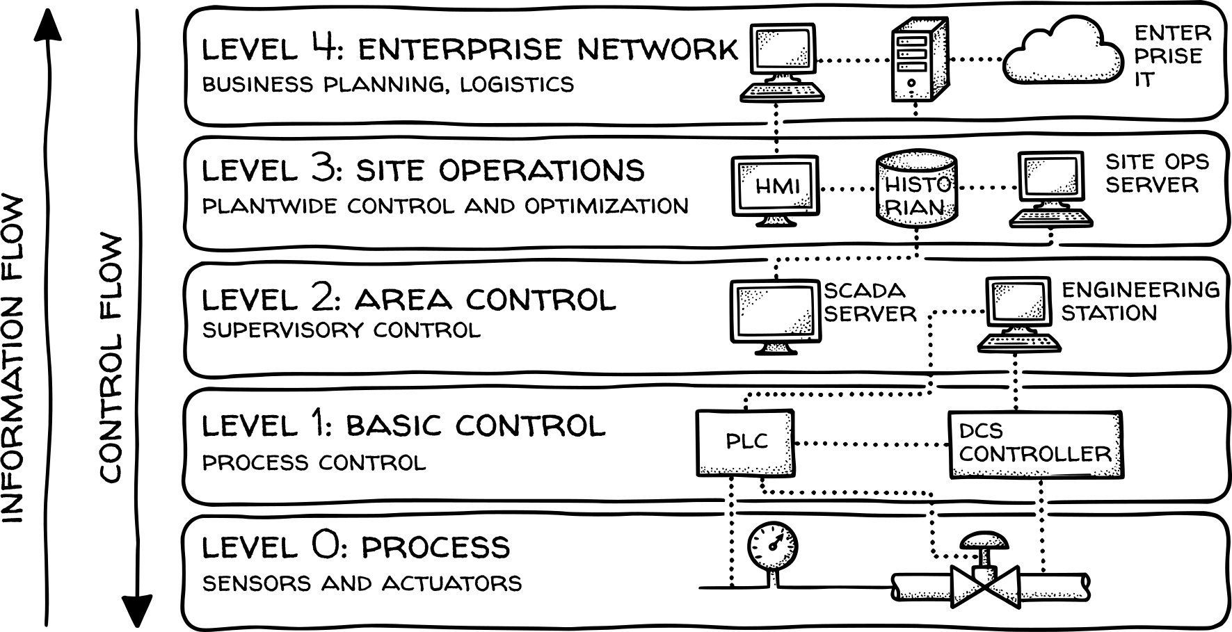
Engineering data hierarchy

  • Level 4 (Enterprise): Business planning (ERP)
  • Level 3 (MES/LIMS): Manufacturing operations, scheduling, QA
  • Level 2 (Control): Real-time control (DCS, PLC)
  • Level 1 (Sensing): Instrumentation, high-freq data
  • Level 0 (Process): Physical equipment

Engineering data hierarchy

  • Levels 0-2 (Lower tier):
    • High volume/velocity
    • Real-time stability focus
    • Short retention (hours-weeks)
  • Levels 3-4 (Upper tier):
    • Lower volume, higher context
    • Production metrics
  • Evolution:
    • Unified Name Space (UNS)
    • Breaking data silos

Diverse engineering data sources

Process operational & experimental

  • Operational: DCS time-series, batch records
  • IoT & Visual: Vibration, acoustic, thermal images
  • Experimental: Pilot plant, bench-scale (validation)
  • Asset data: Maintenance logs, reliability metrics

Engineering & simulation

  • Design: P&IDs, CAD models, specs
  • Properties: Physical & safety data sheets
  • Simulation: Aspen Plus, CFD surrogates
  • Regulatory: Emissions logs, HAZOP reports

Business & contextual

  • Economic: Utility pricing, market data, capital costs
  • Logistics: Inventory levels, raw material transactions
  • Unstructured: Operator logs, shift notes, patents

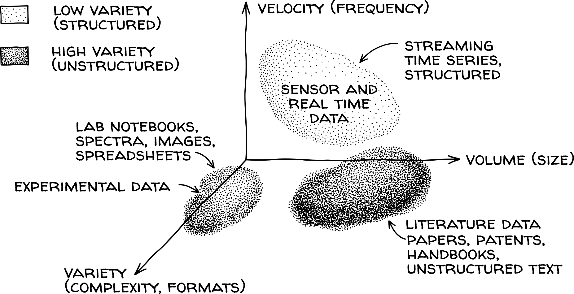
Dimensions of engineering data

  • Volume: GBs of sensor logs to singular design docs
  • Velocity: Millisecond control signals to static reference data
  • Variety: Structured time-series, logs, images, documents
  • Veracity: Calibrated sensors vs. soft sensors (uncertainty)
Dimensions of engineering data

  • Value: Context-dependent (single failure report > routine logs)
  • Lifecycle: Transient errors discarded; regulatory records archived decades
  • Ownership: Fragmented (corporate, personal, public databases)

Data requirements

The choice of modeling strategy determines the data requirements

  • First-principles (Level 3):
    • Engineering parameters (geometry, constants)
    • Source: Static specs or lab systems
  • Data-driven (Levels 1-2):
    • Time-series data
    • Source: Sensors, control loops
    • Issues: Noise, compression artifacts
  • Hybrid:
    • Combines fundamental parameters and operational data

Data characteristics and requirements

Model Type Primary Data Needs Volume Quality
First-principles Fundamental properties, structure Low Very High
Empirical/Regression Training/validation sets Medium High
Data-driven/ML Historical operating data Very High Medium
Hybrid All of the above High High

Data integration challenges

Modelers rarely receive analysis-ready data.

  • Incompatible formats:
    • Sensors: High-freq CSV, unsynchronized timestamps
    • Experiments: Excel, handwritten notebooks
    • Visual: Photos, videos
    • Properties: Static graph images (require digitization)
    • Context: Unstructured PDF shift logs
  • Task: Programmatic combination (resampling, digitization, parsing)

Terminology: Role in process

  • Inputs (Independent variables):
    • Manipulated variables: Actively controlled (valves, pumps)
    • Disturbances: Unmeasured/uncontrolled (ambient temp, feed composition)
  • Outputs (Dependent responses):
    • Result from process (quality, conversion)
  • State variables:
    • Describe internal system state (concentrations, internal temps)
  • Parameters:
    • System constants (heat transfer coeff, dimensions)

Terminology: Measurability

  • Measured variables:
    • Directly observed (sensors, meters)
  • Inferred/Estimated variables:
    • Calculated from others (soft sensors)
  • Unmeasured variables:
    • Neither measured nor inferred
    • Influence process (catalyst activity, fouling)

Terminology: Temporal behavior

  • Static variables:
    • Time-invariant (specs, setpoints)
  • Dynamic variables:
    • Time-varying (profiles, trajectories)
  • Stochastic variables:
    • Random behavior (noise, uncertainty)

Terminology: Data usage

  • Training data:
    • Used to fit model parameters
  • Validation data:
    • Used to tune hyperparameters (prevent overfitting)
  • Test data:
    • Final evaluation on unseen data
  • Inference/Production data:
    • Real-time data for deployment predictions

Structural properties

  • Drift:
    • Changes in data properties (sensor calibration, catalyst deactivation)
  • Autocorrelation:
    • Correlation with past values (violates independence assumption)
  • Collinearity:
    • Strong linear relationships between inputs (destabilizes coefficients)
  • Bias:
    • Systematic offset (calibration error, selection bias)

ML terminology in process context

  • Features (Inputs):
    • Carry physical units and constraints
  • Overfitting:
    • Fitting noise/training data too closely
    • Can violate physical laws outside training range
  • Cross-validation:
    • Estimating performance by partitioning
    • Issues: Autocorrelation (requires forward-chaining splits)

Data quality issues

Raw data is rarely clean. Sources of error include:

  • Operational data:
    • Sensor faults, multi-rate sampling, timestamp drift
  • Lab/Experimental data:
    • Non-random missing values, transcription errors
  • Engineering/Simulation data:
    • Model-reality mismatch, version control
  • Business data:
    • Labeling/metadata errors

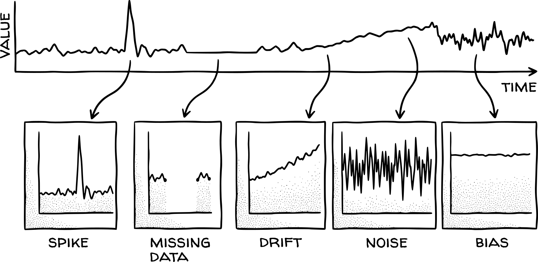
Anomalies in time-series data

  • Spike: Transient excursion (interference)
  • Missing data: Gaps (outages)
  • Drift: Slow shift (fouling)
  • Noise: Rapid fluctuations (turbulence)
  • Bias: Constant offset (calibration)

Data preprocessing

Raw data requires conditioning before modeling.

  • Tasks:
    • Filling gaps
    • Handling outliers
    • Aligning time series
    • Identifying operating regimes
  • Historian compression:
    • Exception-based (deadband)
    • Reduces storage but creates irregular timestamps
    • Goal: Extract raw event stream

Signal reconstruction

Most modeling algorithms expect equal time intervals (constant \Delta t).

  • Sample interval: Depends on dynamics (thermal vs pressure)
  • Reconstruction methods:
    • Zero-order hold: Forward-fill (setpoints, valves)
    • Linear interpolation: Connect points (continuous variables)
  • Note: Prefer raw event stream to control reconstruction

Multirate data alignment

Industrial sources have different rates (seconds vs shifts).

  • Alignment: Align onto common time grid
  • Causal alignment:
    • Avoid future leakage (e.g., using 10:00 lab for 08:00 data)
    • Lag slow variables to match available information
    • Model explicit delays (analyzers)

Steady-state detection

Assumption: Process mean/variance are constant.

  • Violations: Startups, transitions, upset recoveries
  • Detection methods:
    • Rolling variance: Threshold check
    • R-statistic: Variance ratio (R \approx 1 steady)
  • Action: Exclude non-steady periods from training

Outlier detection

Points deviating markedly from expected range.

  • Causes: Transients, artifacts, errors
  • Detection:
    • Univariate: 3-sigma, physical limits
    • Multivariate: PCA, clustering (unusual combinations)
  • Handling: Remove, interpolate, or flag (audit trail required)

Preprocessing validation

No pipeline should be trusted without validation.

  • Visual check: Plot raw vs processed
  • Physics check: Mass and energy balances
  • Sensitivity: Compare results from different methods
  • Reproducibility: Version control pipeline

Data-driven modeling workflow

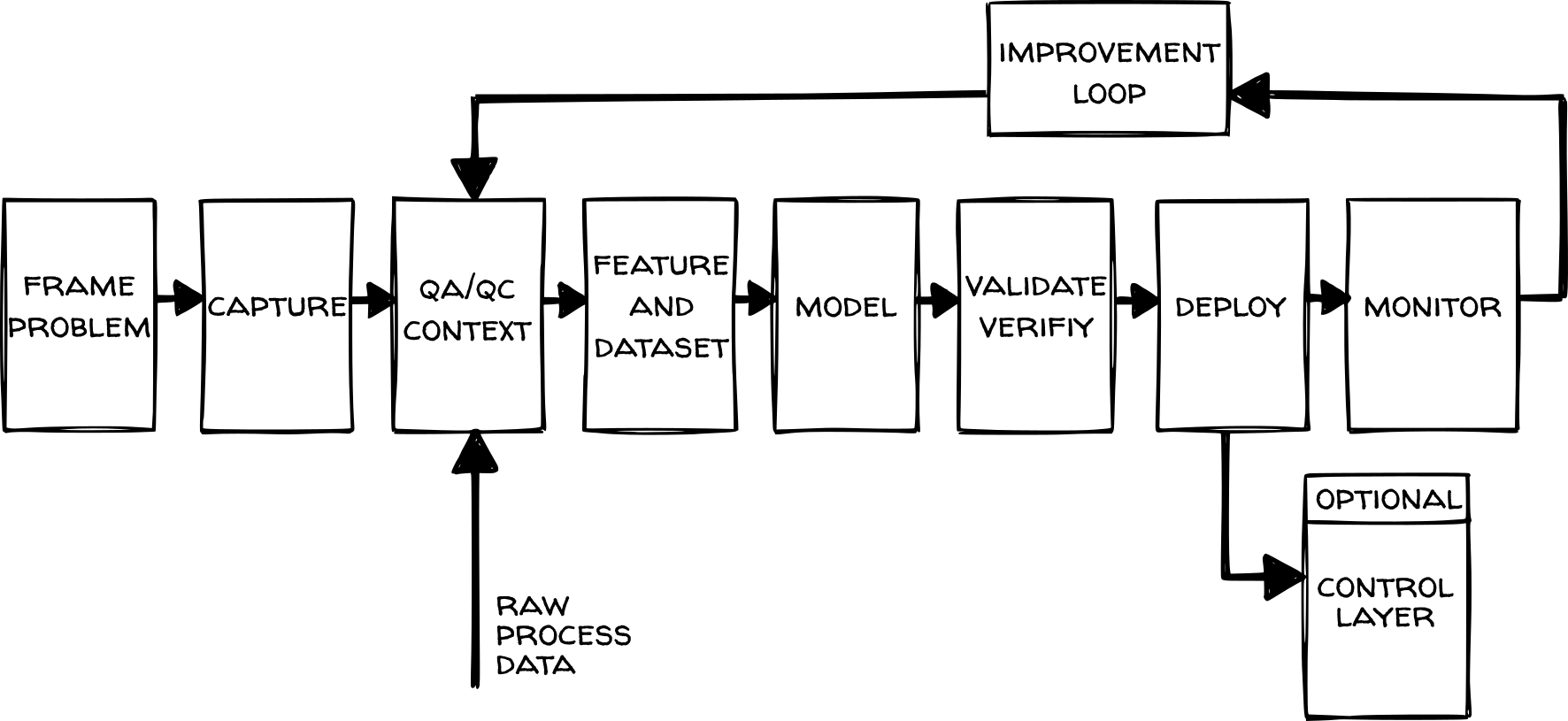
Workflow: Phase 1-4

  • Problem framing: Objective, prediction horizon, KPIs
  • Data collection: Signals, sources, context tags
  • QA/QC: Tag mapping, timestamps, bad data removal
  • Feature construction: Resampling, dataset splitting

Workflow: Phase 5-8

  • Development: Occam’s razor (simplest effective model)
  • Validation: Time-based splitting, backtesting
  • Deployment: Integration into production
  • Monitoring: Track health, trigger improvement loops

Recap

  • Data landscape: Diverse sources (Level 0-4) with varying rates, quality, and imperfections.
  • Conditioning: Requires reconstruction (zero-order/linear), causal alignment, and cleaning.
  • Filtering: Outliers and non-steady periods must be identified and handled.
  • Validation: Verify data quality via visual inspection and physics balances.
  • Workflow: Development follows a structured 8-phase lifecycle from framing to monitoring.

Which is the greater barrier to effective modeling: The Availability of data or the Quality of data?

Process characterization

Process characterization vs. dynamics

  • Chemical processes are rarely static (disturbances, feedback).
  • Characterization: Systematic analysis of behaviors.
    • What variables matter?
    • Is the process stable?
  • Dynamics: Time-dependent behavior.
    • How does the system transition states?
    • How does it respond to disturbances?

Identifying dynamics

  • Classical approach:
    • First principles transfer functions
    • Rigorous step tests
  • Data-driven approach:
    • Interrogating historical data
    • Searching for dynamic “fingerprints” (time constants, dead times)
    • Challenge: Handling noise and irregular sampling

First look: Exploratory Data Analysis

  • Motivation: Visualization prevents modeling statistical artifacts.
    • Distinguish upsets from instrument failures.
    • Reveal operating regimes.
  • EDA (Tukey):
    • Graphical techniques to discover structure.
    • Contrast with hypothesis testing (which confirms structure).

Visualizing time-series structure

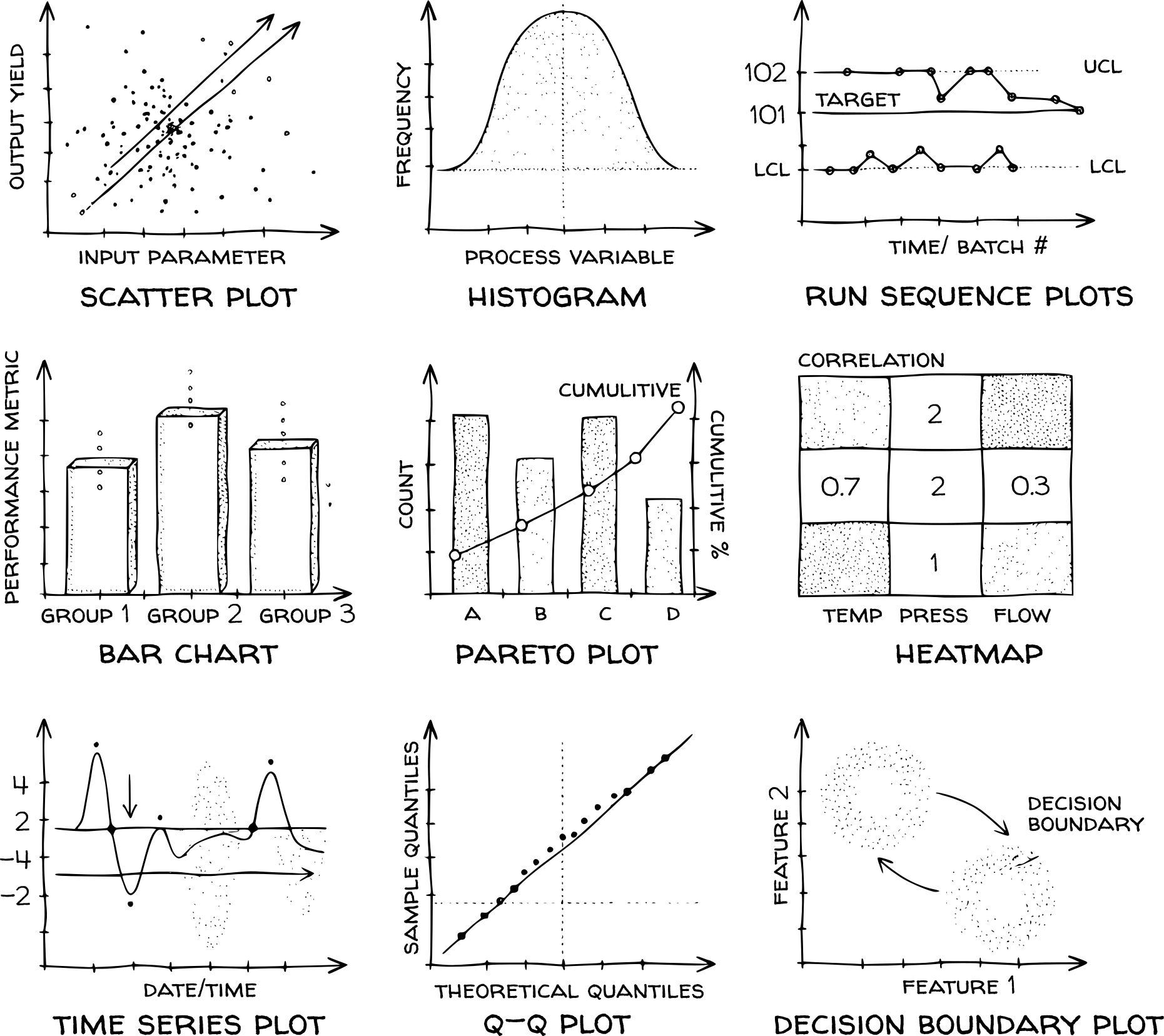
Key EDA plots

  • Run sequence: Shifts in mean/noise, outliers, frozen sensors.
  • Pareto: Rank factors by importance (80/20 rule).
  • Correlation matrix: Pairwise dependencies, collinearity.
  • Lag plots: Detect autocorrelation (Y_i vs Y_{i-1}).
  • Autocorrelation (ACF): Quantify process memory.
  • Box plots: Distributions, outliers > 1.5 IQR.
  • Q-Q plots: Test Gaussian assumption (normality).

Example: CSTR with cooling jacket

Process description:

  • System: Continuous Stirred Tank Reactor (CSTR)
  • Goal: Visualize correlation of inputs to outputs
  • Variables:
    • Inputs (Setpoints): C_{A,in}, T_{in}
    • Measured Outputs: C_A (outlet conc.), T (reactor temp), T_c (coolant temp)

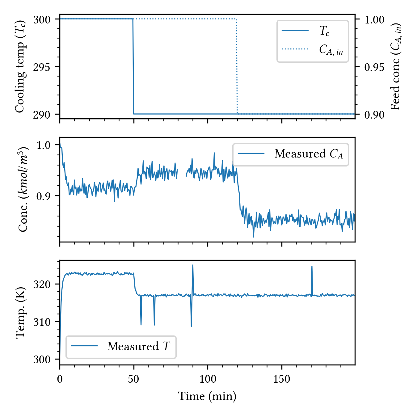
CSTR Data Inspection

  • Nominal start: Steady operation.
  • Step changes:
    • t=50: Cooling temp drop (T_c \downarrow \rightarrow T \downarrow \rightarrow C_A \uparrow)
    • t=120: Feed conc drop (C_{A,in} \downarrow \rightarrow C_A \downarrow)
  • Data quality issues:
    • High-frequency noise (needs filtering)
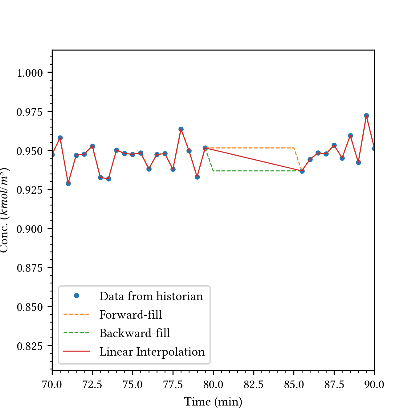
    • Data gap at t=80 (needs imputation)
    • Outlier spikes (needs removal)

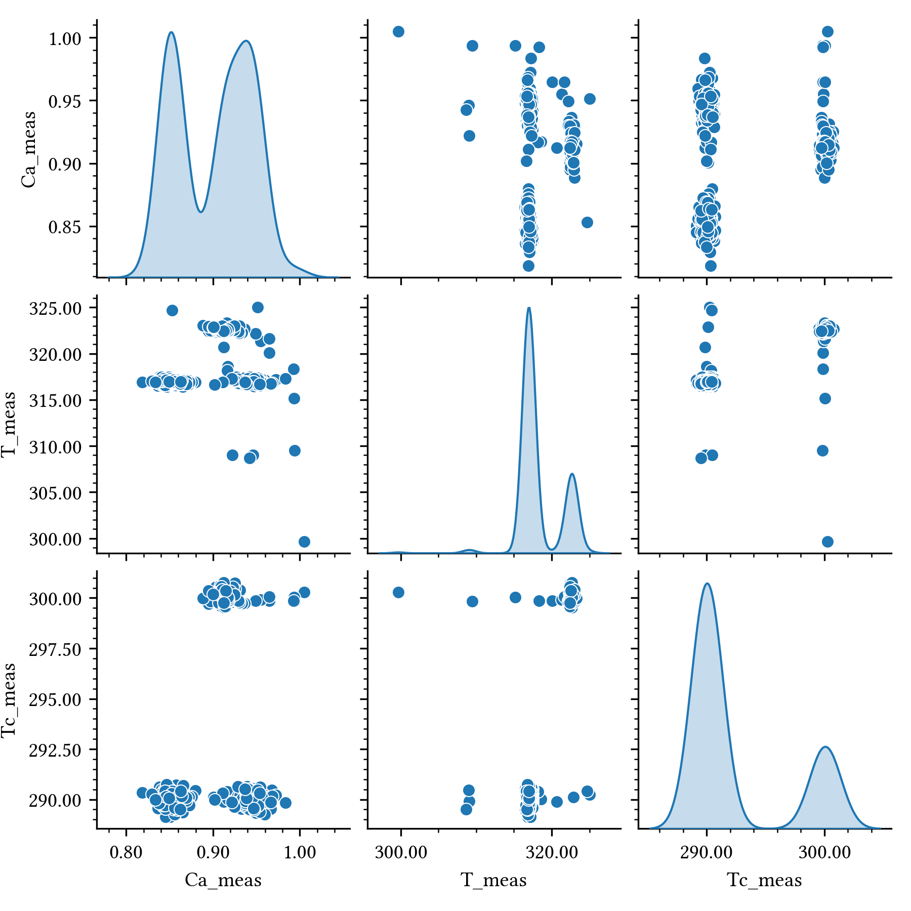
Scatter matrix (pair plot)

  • Grid of scatter plots for all variables (diagonals show distributions).
  • Reveals non-obvious coupling and operating regime shifts.
  • Exposes static correlation structure vs temporal trends.

CSTR scatter matrix features

  • Bimodality: KDE shows two operating regimes.
  • Cluster separation: Three clusters from distinct phases.
  • Step signature: Vertical bands at T_c = 290, 300 K.
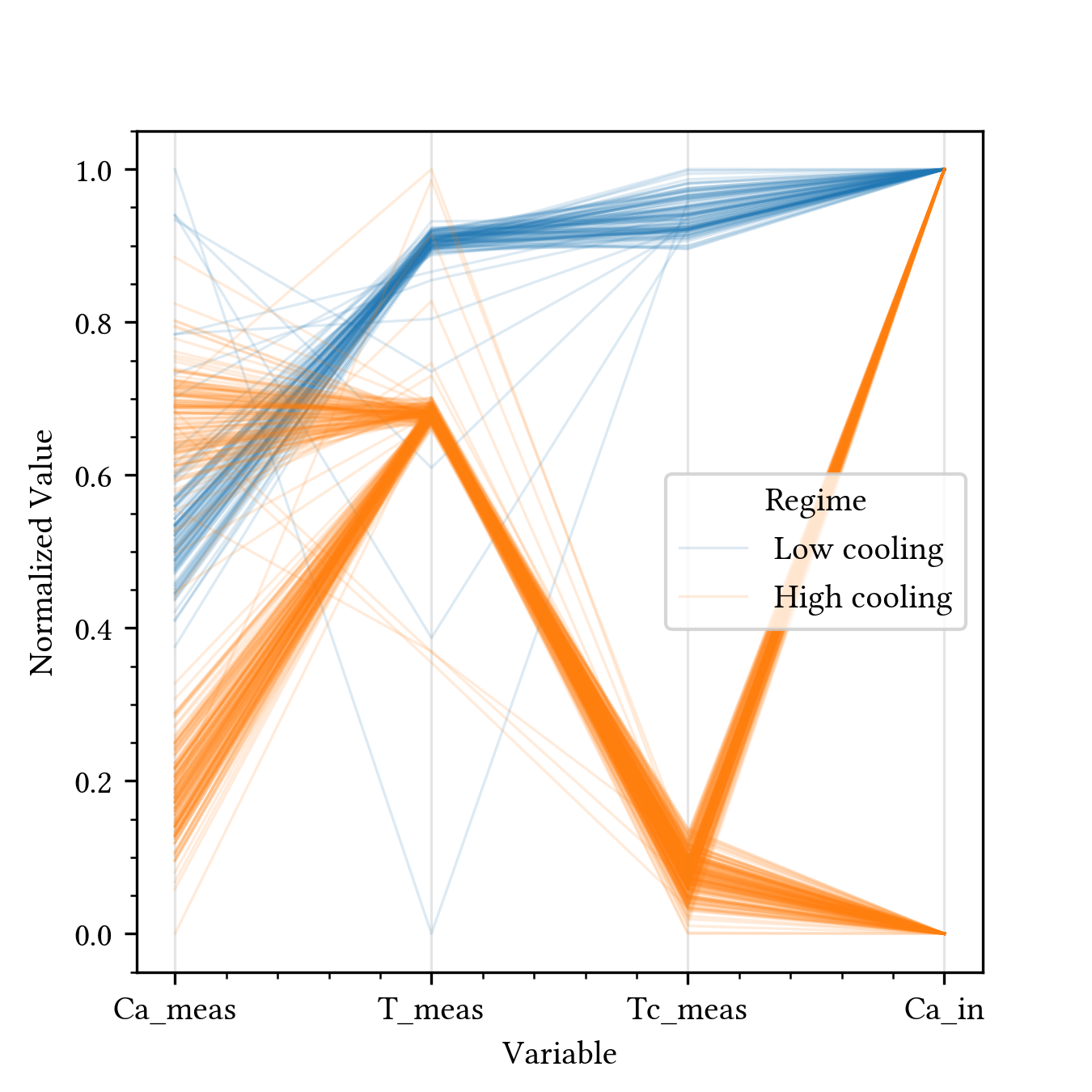
Parallel coordinates plot

  • Maps each row as a line through vertical axes.
  • Excellent for visualizing operating regimes (4+ variables).
  • Bundle structure identifies regime transitions:
    • Low cooling: High T_c, T; low C_A
    • High cooling: Opposite pattern

Missing value imputation

  • Sources: Sensor maintenance, network latency, compression.
  • Strategies:
    • Forward-fill: Zero-order hold (creates steps).
    • Backward-fill: Non-causal (uses future data).
    • Linear interpolation: Preferred for continuous processes.
  • Caution: If gap > time constant, discard segment.
Spike removal methods

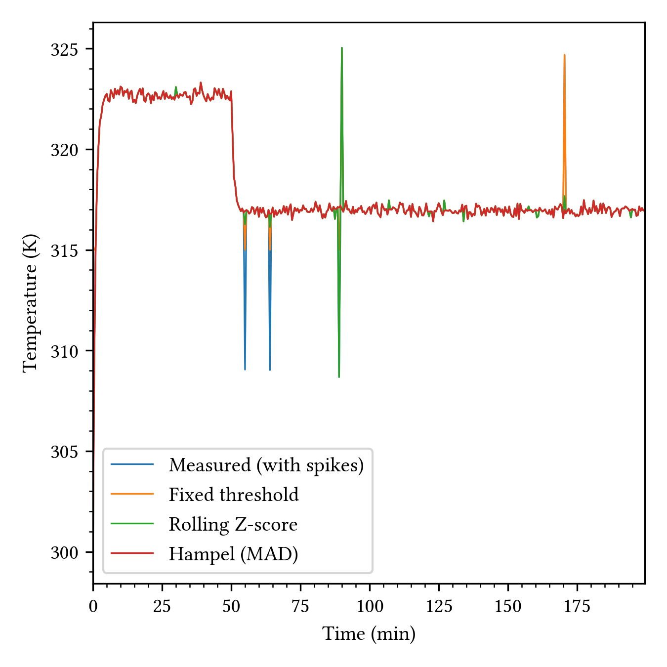
  • Spikes bias model parameters and error statistics.
  • Two approaches: Clipping (boundary) vs Replacement (local value).
Fixed thresholding

  • Global clip: y_{clipped} = \min(\max(y_i, y_{min}), y_{max})
  • Disadvantage: Ignores local context (false positives/negatives).

Rolling Z-score

  • Uses local mean \mu_{i,N} and std \sigma_{i,N}: y_{filtered} = \begin{cases} \mu_{i,N} & \text{if } |y_i - \mu_{i,N}| > k \cdot \sigma_{i,N} \\ y_i & \text{otherwise} \end{cases}
  • Threshold: k=3 (3-sigma rule).
  • Issue: Outliers inflate std (masking).

Hampel filter (most robust)

  • Uses median m_{i,N} and median absolute deviation (MAD) (robust to outliers): y_{filtered} = \begin{cases} m_{i,N} & \text{if } |y_i - m_{i,N}| > k \cdot (c \cdot MAD_{i,N}) \\ y_i & \text{otherwise} \end{cases}
  • Scaling constant: c \approx 1.4826 (aligns MAD with \sigma).
  • 3-sigma threshold: 99.73% confidence (0.3% false positive rate).

Spike removal comparison

  • Fixed thresholding:
    • Clips to global bounds.
    • Fails during regime shifts (misses new-regime spikes).
    • May truncate legitimate process data.
  • Rolling Z-score:
    • Accounts for local variation.
    • Susceptible to masking: Large outliers inflate std.
    • At t=90 min: Outlier masks itself.
  • Hampel filter:
    • Uses median and MAD (robust to outlier magnitude).
    • Precise pruning without spurious artifacts.
    • Best for high-noise environments.

Noise filtering methods

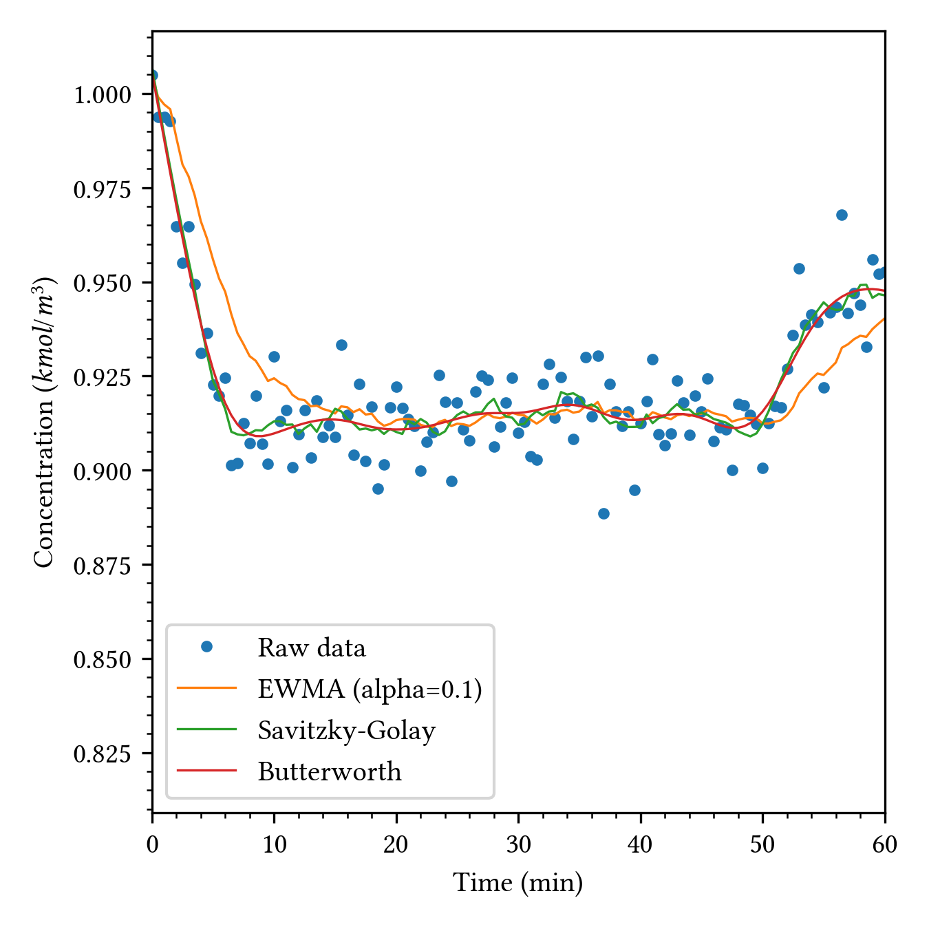
  • Moving average (MA): Suppresses noise, introduces lag.
  • EWMA: Recursive, weights recent data, balances smoothing and responsiveness.
  • Median filter: Robust for non-Gaussian noise and spikes.
  • Savitzky-Golay: Local polynomial, preserves peaks and derivatives.
  • Butterworth: Precise frequency cutoff control.
  • Kalman: Optimal when process model available.
  • Wavelet: Multi-resolution for non-stationary signals.
Filter comparison

  • EWMA:
    • Phase lag (shifts signal right).
    • Real-time recursive implementation.
  • Savitzky-Golay:
    • Zero lag, preserves higher-order moments.
    • Sensitive to local outliers.
  • Butterworth (filtfilt):
    • Sharp cutoff, zero phase shift.
    • Requires batch processing.

Data reconciliation

  • Problem: Raw measurements contain errors (bias, noise).
    • Models trained on biased data learn instrument faults, not physics.
    • Bias degrades predictions when sensors are recalibrated.
  • Solution: Adjust measurements to satisfy conservation laws.
    • Enforces mass/energy/momentum balances.
    • Requires redundancy (more measurements than equations).
  • Benefit:
    • Physics-consistent training data.
    • Robust models for control/optimization.

Mathematical formulation

  • Optimization problem: Constrained weighted least-squares.
    • Minimize: Weighted sum of squared adjustments.
    • Subject to: Balance equations (linear/nonlinear).
  • Key challenges:
    • Scale: thousands of variables/constraints.
    • Covariance estimation: serial/cross-correlation affects weights.
    • Decomposition: Graph-theoretic methods partition large problems.

Gross error detection

  • Gross errors: Systematic bias or sensor failure.
    • Must be removed before reconciliation (invalidates statistics).
  • Workflow:
    1. Detect gross errors (statistical tests).
    2. Eliminate/isolate faulty sensors.
    3. Reconcile remaining random errors.
  • Constraints: Use fundamental laws (mass/energy), avoid empirical correlations.

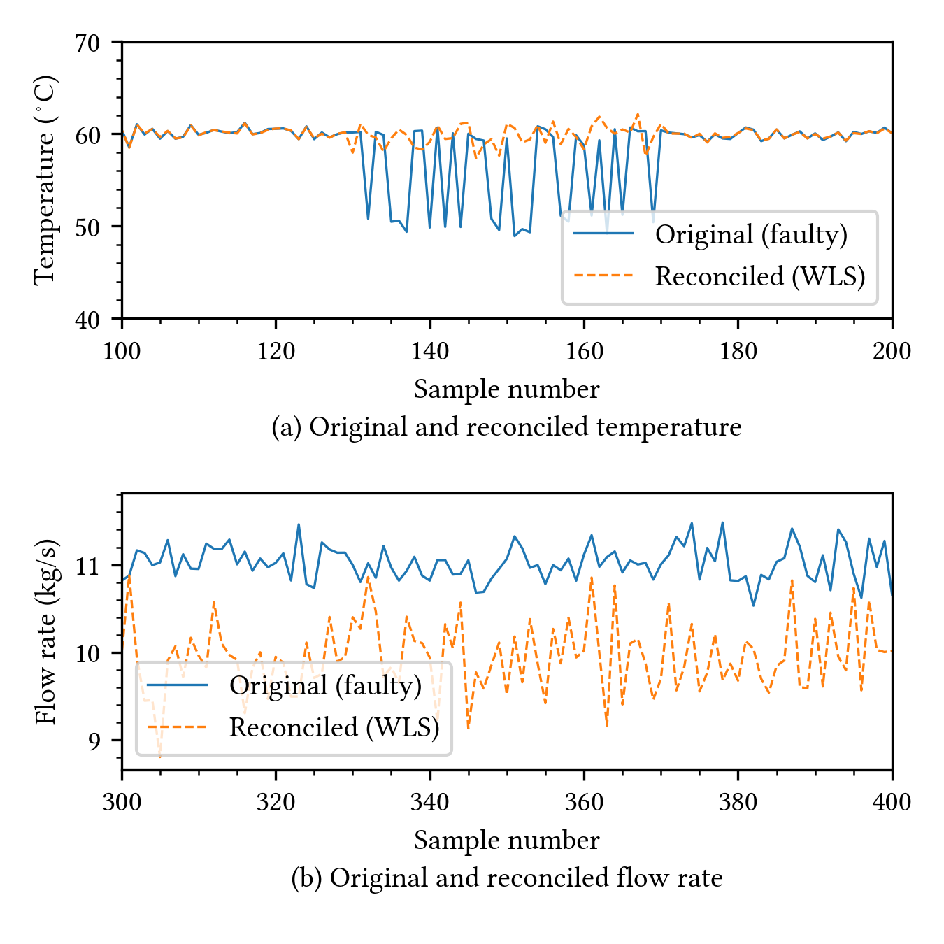
Example: Heat exchanger energy balance

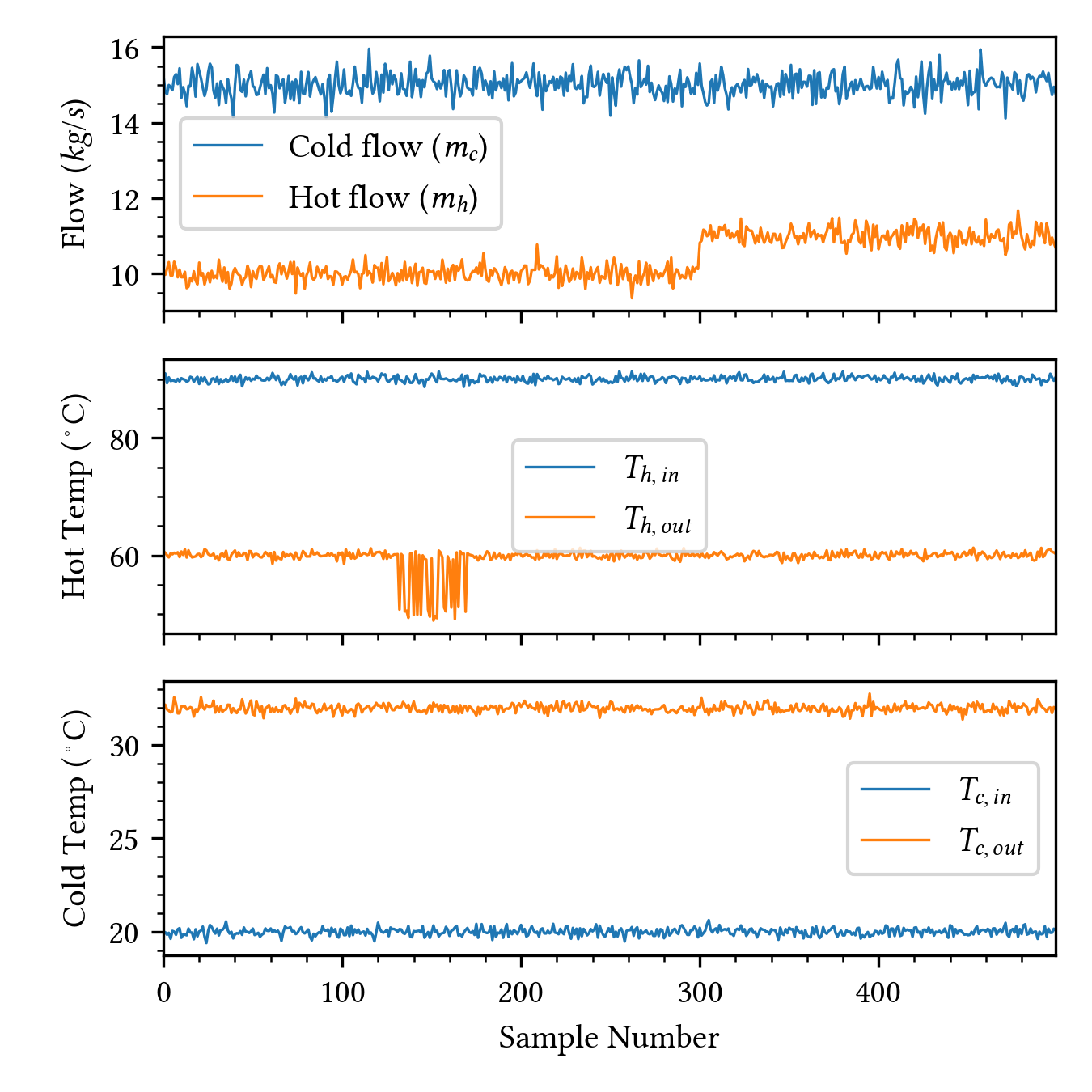
  • Counter-current heat exchanger (Hot/Cold streams).
  • Measurements: Flow (m), Temp (T_{in}, T_{out}).
  • Faults:
    • Stuttering T_{h,out} (samples 130-170).
    • Sudden bias in m_h (sample 300+).
  • Visual check: T_{out} flat despite m_h jump? Suspicious.
Physics-based residuals

  • Z-score (z = (x - \mu) / \sigma):
    • Measures distance from mean in standard deviations.
    • Only flags extreme values (e.g., |z| > 3).
    • Failure mode: Misses sensor drift within normal operating range.
  • Physics reveals all: Energy balance must close. m_h C_{p,h} (T_{h,in} - T_{h,out}) = m_c C_{p,c} (T_{c,out} - T_{c,in})
  • Residual (R): Difference between calculated duties.
    • R \approx 0 (normal).
    • R \neq 0 (fault/leak).

Gross error reconstruction

  • Identify fault: High residual contribution.
    • Set weight \sigma_i \to \infty.
  • Reconstruct: Solve optimization with healthy sensors.
  • Result:
    • Filters stuttering (T_{h,out}).
    • Reconciles bias (m_h) to physics.

Automated steady-state detection

  • Goal: Establish baseline behavior for:
    • Data reconciliation (balances close).
    • Gain estimation (K).
    • Model initialization.
  • Method: Aumated rolling variance.
    • Steady if variance < threshold.
  • Constraint: Zero accumulation (variables constant on average).

Steady-state detection example

  • Step change: T_c drops (300 K to 290 K).
  • Process settles to new steady state.
  • Gain (K): Sensitivity of reactor temp. K = \frac{\Delta T}{\Delta T_c} = \frac{T_{new} - T_{old}}{290 - 300}
  • Positive gain: Strong coupling to jacket.
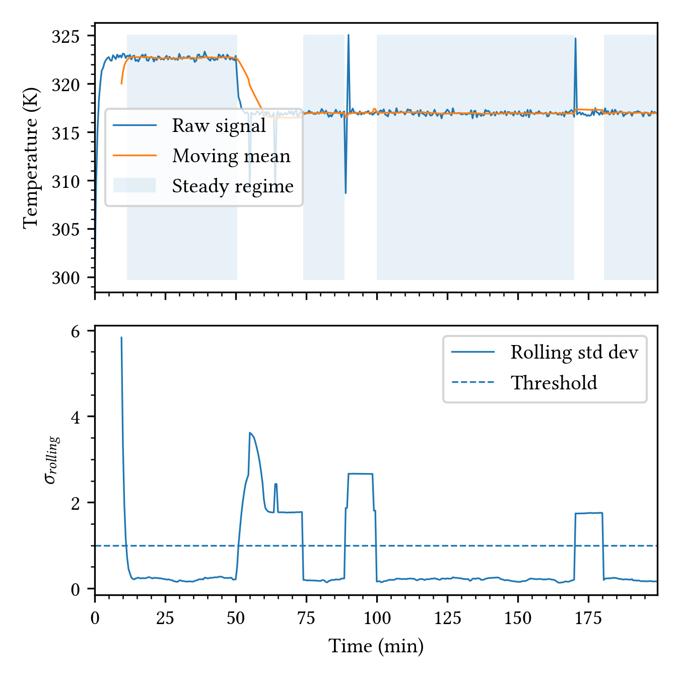
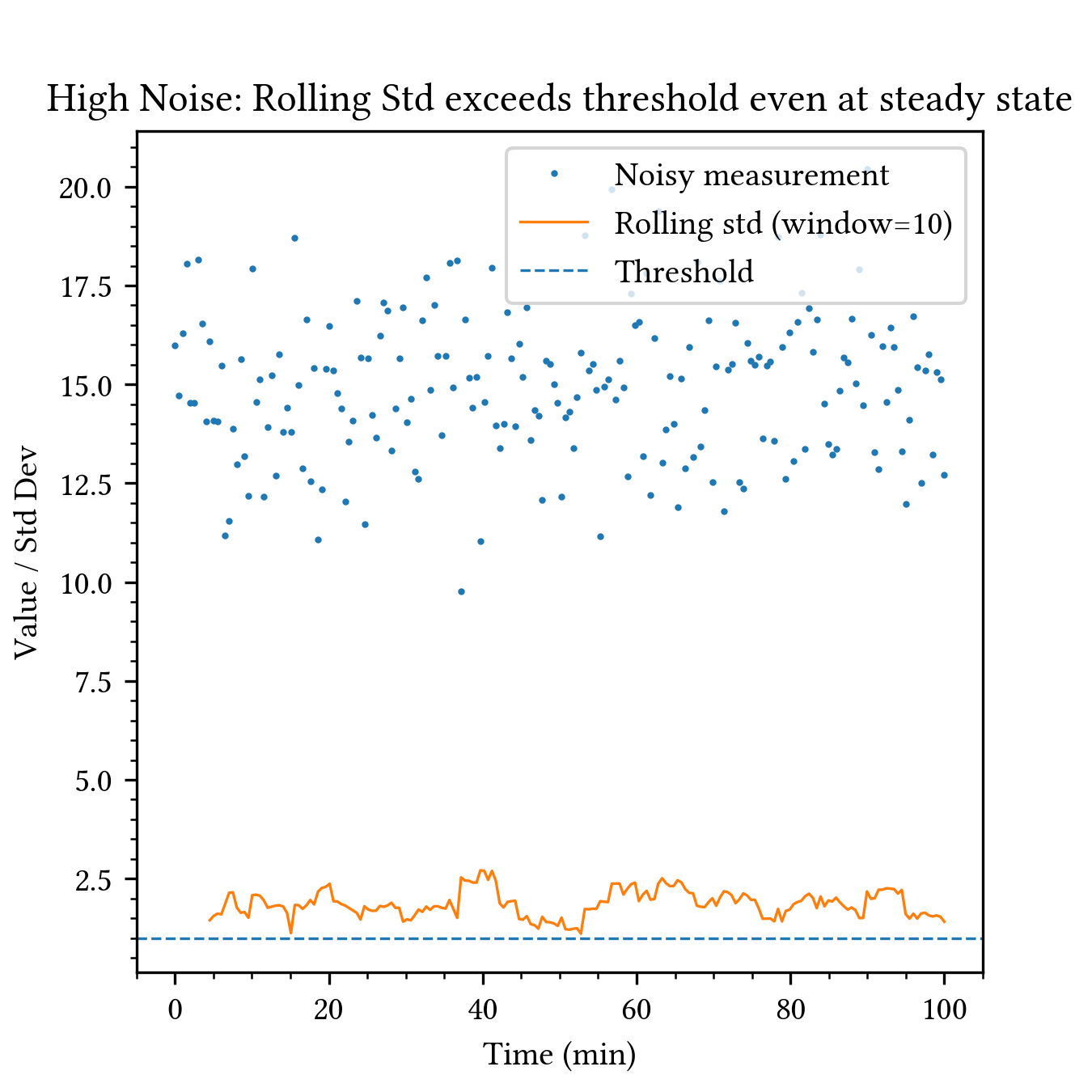
Challenge: High noise

  • Issue: High noise masks steady state.
    • Rolling std dev exceeds threshold.
    • Result: False positives (unsteady).
  • Fix:
    • Increase window size (averaging).
    • Filter data (EWMA/Butterworth).

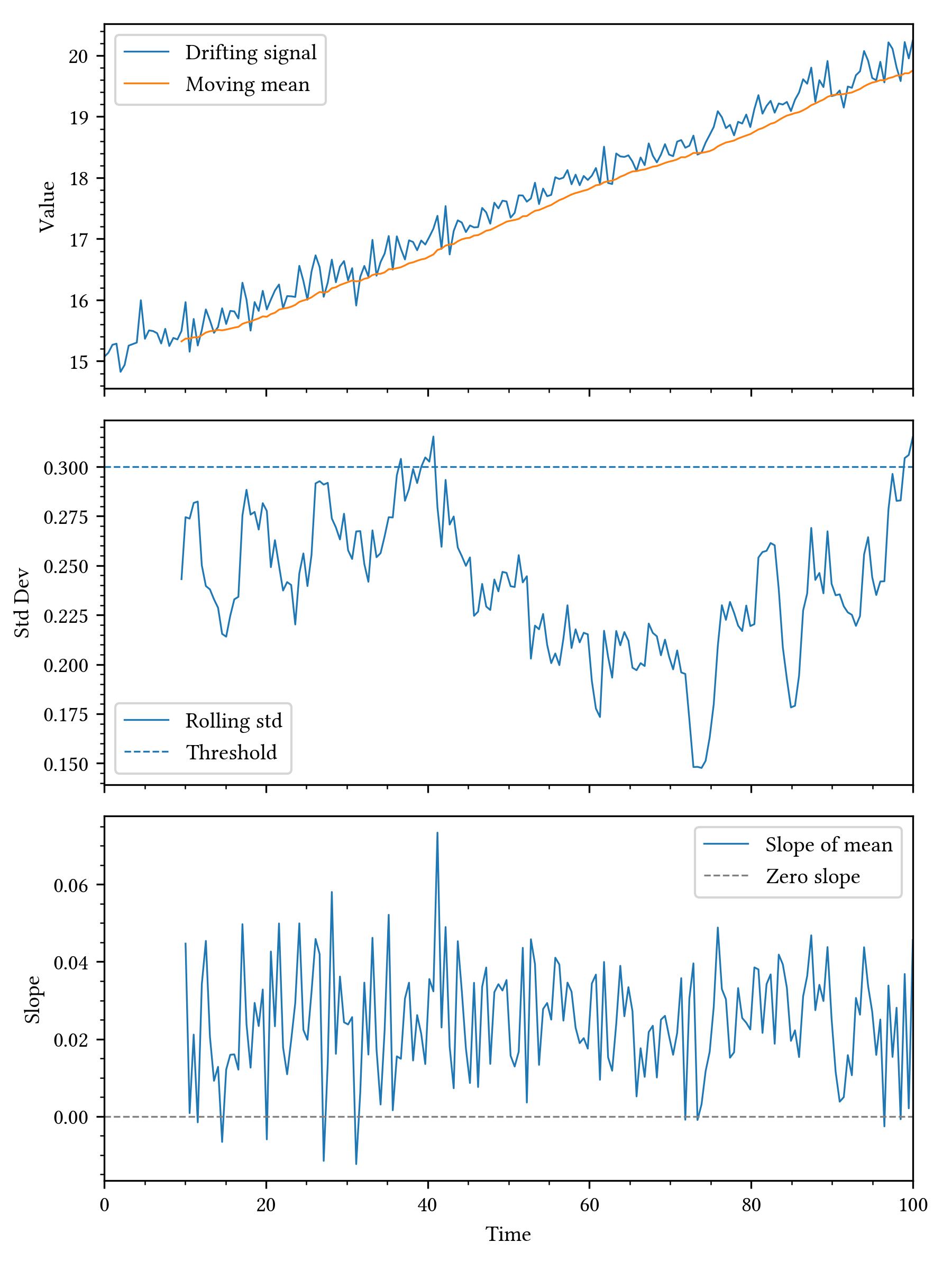
Challenge: Process drift

  • Issue: Slow degradation (fouling/poisoning).
    • Low variance (appears steady).
    • Non-zero slope (drifting).
  • Fix: Monitor both variance and slope.
    • True steady state: Low variance + Zero slope.
Stationarity (ADF test)

  • Stationarity: Constant statistical properties (mean/variance).
  • Augmented Dickey-Fuller (ADF) test:
    • Regress first difference \Delta y_t: \Delta y_t = \alpha + \beta t + \gamma y_{t-1} + \sum_{j=1}^k \delta_j \Delta y_{t-j} + \epsilon_t
    • Test coefficient \gamma: If \gamma = 0 (unit root) \rightarrow Non-stationary.

Interpreting ADF results

  • ADF Statistic: t_{ADF} = \hat{\gamma} / SE(\hat{\gamma}).
  • P-value: Probability of observing t_{ADF} if process is non-stationary. p = \int_{-\infty}^{t_{ADF}} f_{DF}(x) dx
  • Decision:
    • Low p-value (< 0.05): Stationary (steady).
    • High p-value: Non-stationary (drifting).

Process dynamics

Dynamic characterization

  • Goal: Extract time-based descriptors from trajectories.
  • Approaches:
    • Phenomenological: Physical params, good for control/extrapolation.
    • Data-driven: Robust to artifacts/noise, reveals regime changes.
  • Complementary:
    • Data-driven finds horizons/lags.
    • Mechanistic provides constraints.

Autoregressive (AR) model

  • Output depends only on its own history (system memory).
  • Useful when inputs unavailable or constant. y(k) = \sum_{i=1}^{n_a} a_i y(k-i) + e(k)
  • n_a: Model order (persistence).

AR with exogenous inputs (ARX)

  • Adds measured inputs (driving forces) to AR structure. y(k) = \sum_{i=1}^{n_a} a_i y(k-i) + \sum_{j=1}^{n_b} b_j u(k-j-n_k) + e(k)
  • n_b: Input lags.
  • n_k: Transport delay (dead time).

ARMAX model

  • Adds structure to noise term (unmeasured disturbances). y(k) = \text{ARX terms} + \sum_{m=1}^{n_c} c_m e(k-m) + e(k)
  • Moving Average (MA): Accounts for colored noise.
  • Use when ARX residuals remain autocorrelated.

Model configuration

  • Physical intuition guides order selection:
    • AR order: Process inertia/time constant.
    • Input lags (n_k): Transport delay.
    • MA terms: Oscillatory residuals/unmeasured dynamics.
  • Coefficients map to continuous-time constants and gains.

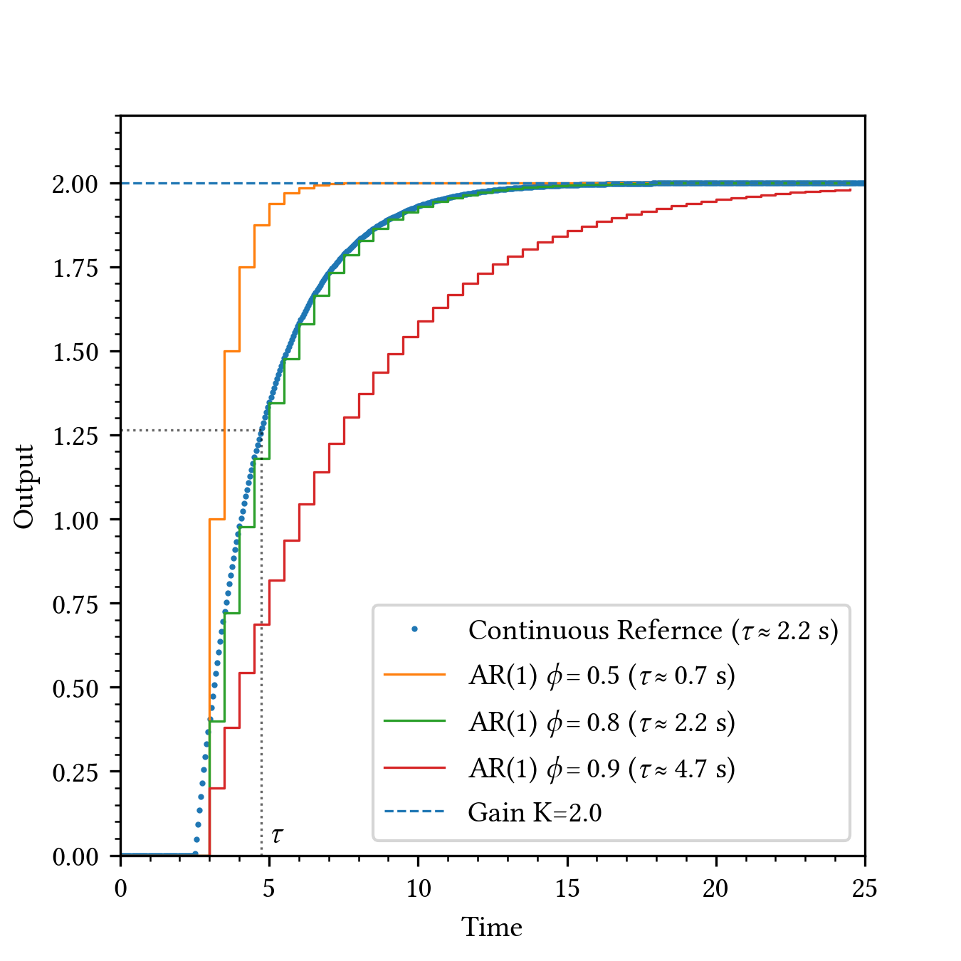
Example: First-order system

  • Physics: Capacity/Inertia (Heating, Filling).
  • Response: Smooth rise to steady state (no overshoot).
  • AR(1) Model: y_t = \phi y_{t-1} + (1-\phi) K u_{t-1}
    • \phi = e^{-\Delta t / \tau}: Autocorrelation coefficient.
    • High \phi \to Slow response (high inertia).
    • Low \phi \to Fast response.

Example: Second-order system

  • Physics: Momentum + Capacity (Fluid oscillation).
  • Response: Overshoot and oscillation (\zeta < 1).
  • AR(2) Model: y_t = \phi_1 y_{t-1} + \phi_2 y_{t-2} + \beta u_{t-1}
  • Roots: Complex conjugates for underdamped systems.
    • \phi_2: Controls decay rate (damping).
    • \phi_1: Controls frequency.

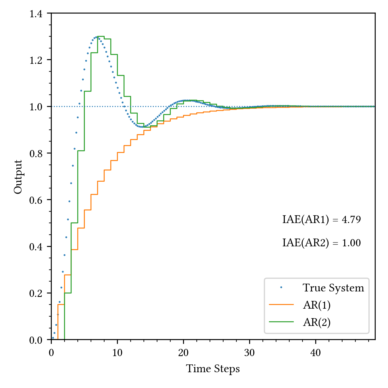
AR(1) vs AR(2) comparison

  • AR(1) cannot capture overshoot.
  • AR(2) matches oscillatory dynamics.
  • Metric: Integral Absolute Error (IAE). \text{IAE} = \sum |y_{true} - y_{model}| \Delta t
  • AR(1) IAE: 4.79
  • AR(2) IAE: 1.0 (Better fit).

Example: System with dead time

  • Dead Time (\theta): Time for material/energy to travel to sensor.
    • e.g., Pipe flow: \tau = Volume/Flow.
    • Difficult to control (no immediate reaction).
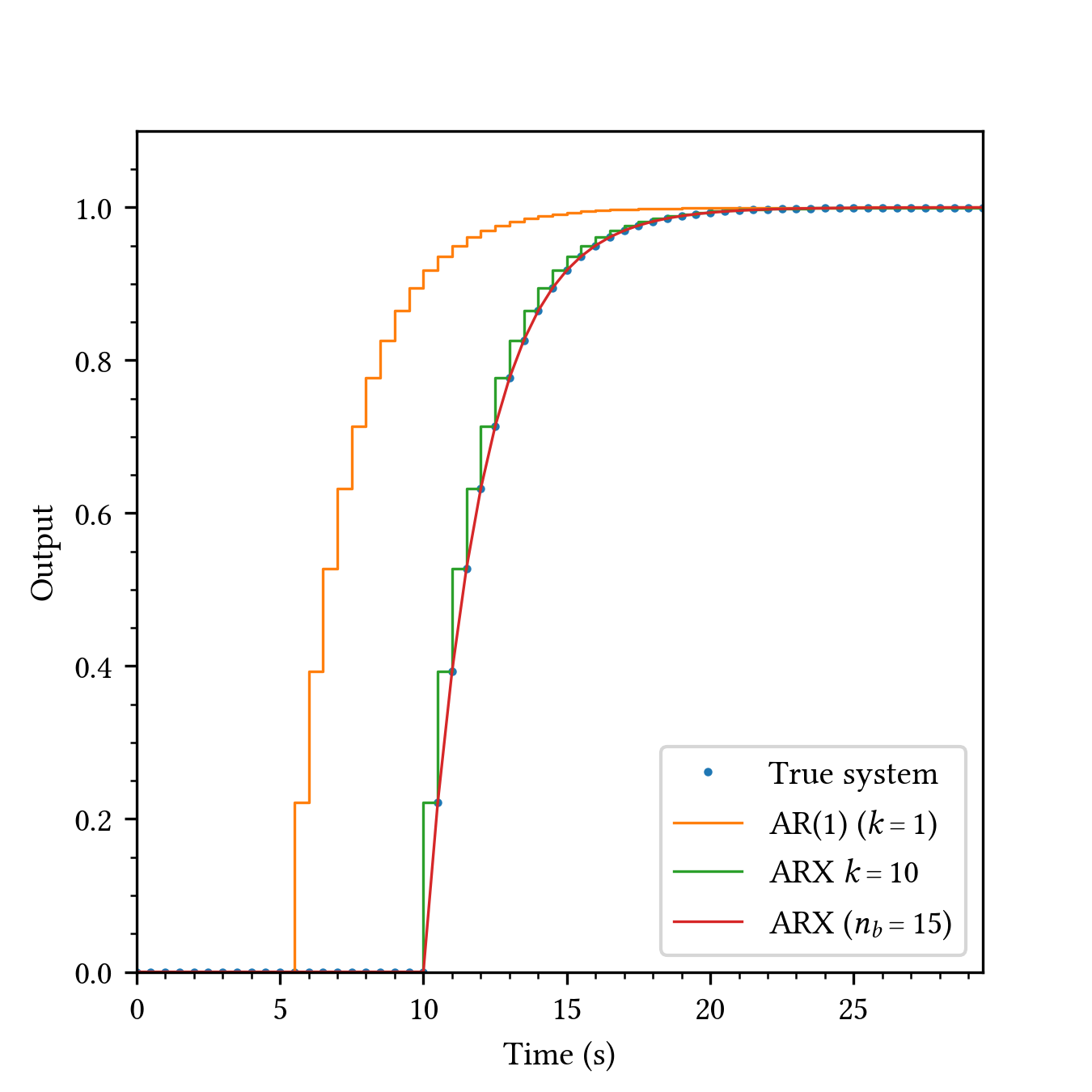
  • Modeling: Use ARX with input delay k = \theta / \Delta t. y_t = a y_{t-1} + b u_{t-k}
  • Pure AR model fails (assumes instant response).

Comparing dead time approaches

  • AR(1): Ignores delay \to Poor initial fit.
  • ARX (Correct k): Physically accurate.
  • High-order ARX: learns delay via zero parameters.
    • Risk: Overfitting, ill-conditioned.
  • IAE values: 100, 1.0, 0.0

Example: Unmeasured disturbances

  • Problem: Process data has drifts/trends (e.g., fouling, ambient temp).
  • ARX failure: Assumes white noise (e_t).
    • Biased parameters (tries to fit drift with input).
  • ARMAX solution: Explicit noise model (e_t \to C(q)e_t). A(q)y(t) = B(q)u(t-k) + C(q)e(t)
  • Separates process dynamics (A, B) from disturbance (C).

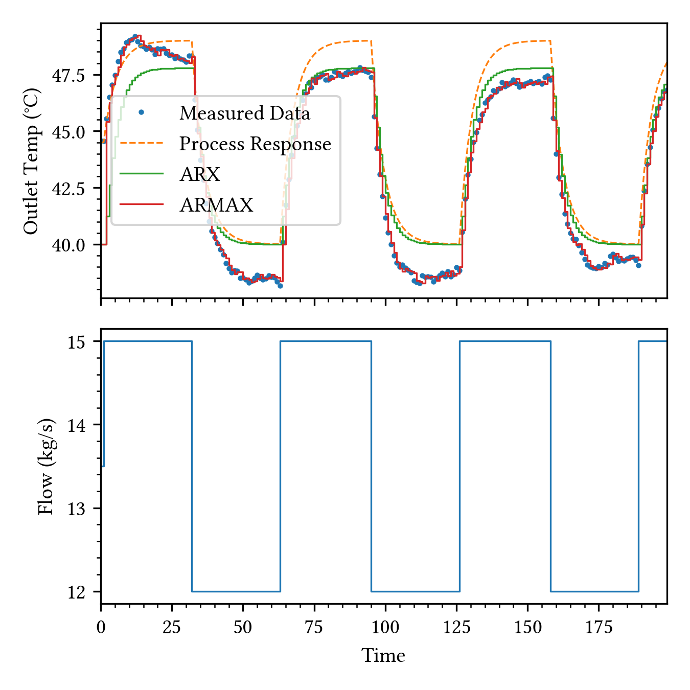
ARX vs. ARMAX results

  • Drift impact: Unmeasured non-stationary disturbance.
  • Process Model: Tracks initially, then fails (IAE = 249.08).
  • ARX: Biased by drift (IAE = 194.87).
  • ARMAX:
    • Captures drift (C(q) term).
    • Fits dynamics (IAE = 31.08).

Comparison of ARX vs ARMAX for unmeasured drifts

Mechanism of ARX failure

  • Assumption: Error e(t) is white noise (independent).
  • Reality: Drift v(t) is non-stationary (autocorrelated). v(t) = v(t-1) + \xi(t)
  • Consequence:
    • Regressor y(t-1) correlates with disturbance v(t).
    • OLS “panics” to reduce error \to shifts poles.
    • Model appears slower (biased parameters).

Estimating ARMAX (ELS)

  • Problem: Noise terms e(t) are unmeasured.
  • Extended Least Squares (ELS): Iterative algorithm.
    1. Fit initial ARX model.
    2. Calculate residuals \hat{e}(t) = y(t) - \hat{y}(t).
    3. Update regressor vector: \phi(t) = [-y(t-1), \dots, u(t-k), \dots, \hat{e}(t-1), \dots]^T
    4. Refit and repeat until convergence.

Trade-off: Accuracy vs. Physics

  • ARMAX: Superior predictor (handles drift).
    • Black box: Parameters mix physics (inertia) + noise.
    • Hard to extract \tau or K.
  • Grey Box: Better for characterization.
    • Detrend data first.
    • Fit simpler, interpretable structure.

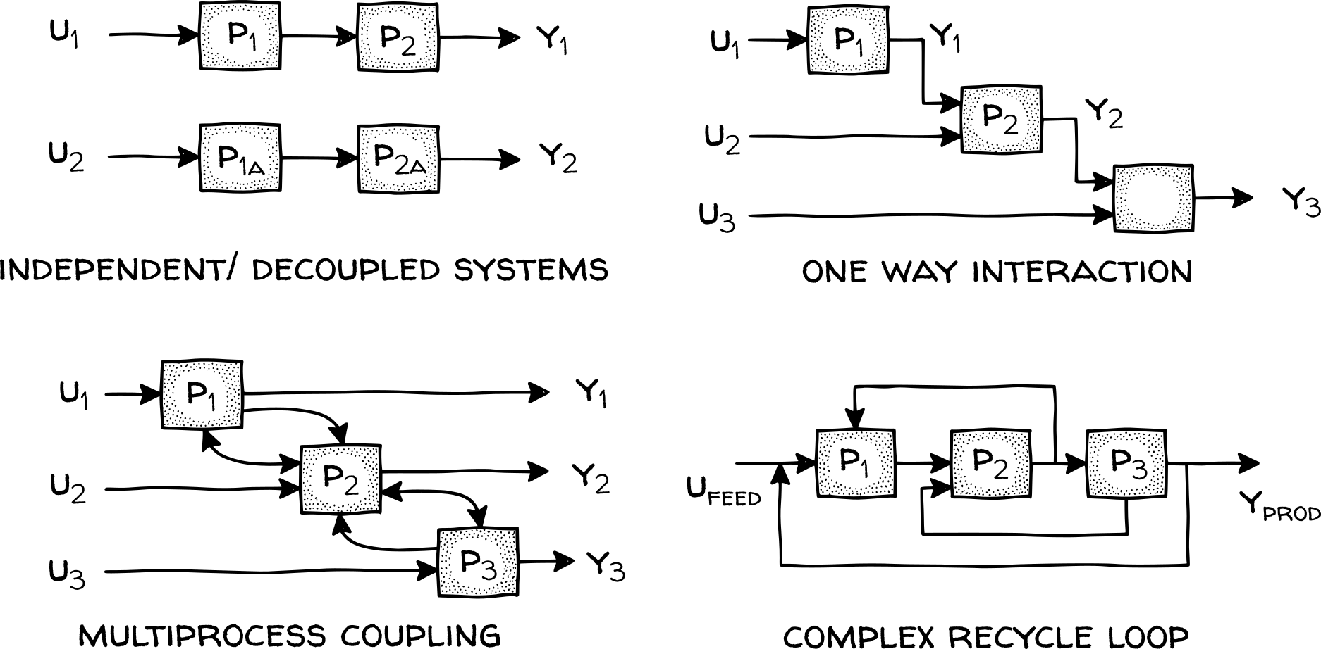
Multi-variable interactions

  • Industrial systems are interconnected networks.
  • Coupling: Shared utilities, feeds, constraints.
  • Patterns:
    • Independent: Isolated loops.
    • One-way: Upstream \to Downstream.
    • Recycle: Circular interactions.

Complex coupling effects

  • Recycle loops:
    • Disturbances return via feedback path.
    • Long autocorrelation tails, non-intuitive correlations.
  • Closed-loop masking:
    • Controllers determine input-output correlation.
    • Hides true process dynamics.
  • Collinearity: Coupled variables move together (hard to separate).

Vector Autoregressive (VAR) models

  • Goal: Learn joint dynamic topology.
  • VAR Model: Regress vector Y_t on its own past. \begin{bmatrix} y_{1,t} \\ \vdots \\ y_{n,t} \end{bmatrix} = \mathbf{A} \begin{bmatrix} y_{1,t-1} \\ \vdots \\ y_{n,t-1} \end{bmatrix} + \dots
  • Granger Causality:
    • If a_{ij} \neq 0: Variable j helps predict i.
    • Maps the process flow sheet from data alone.

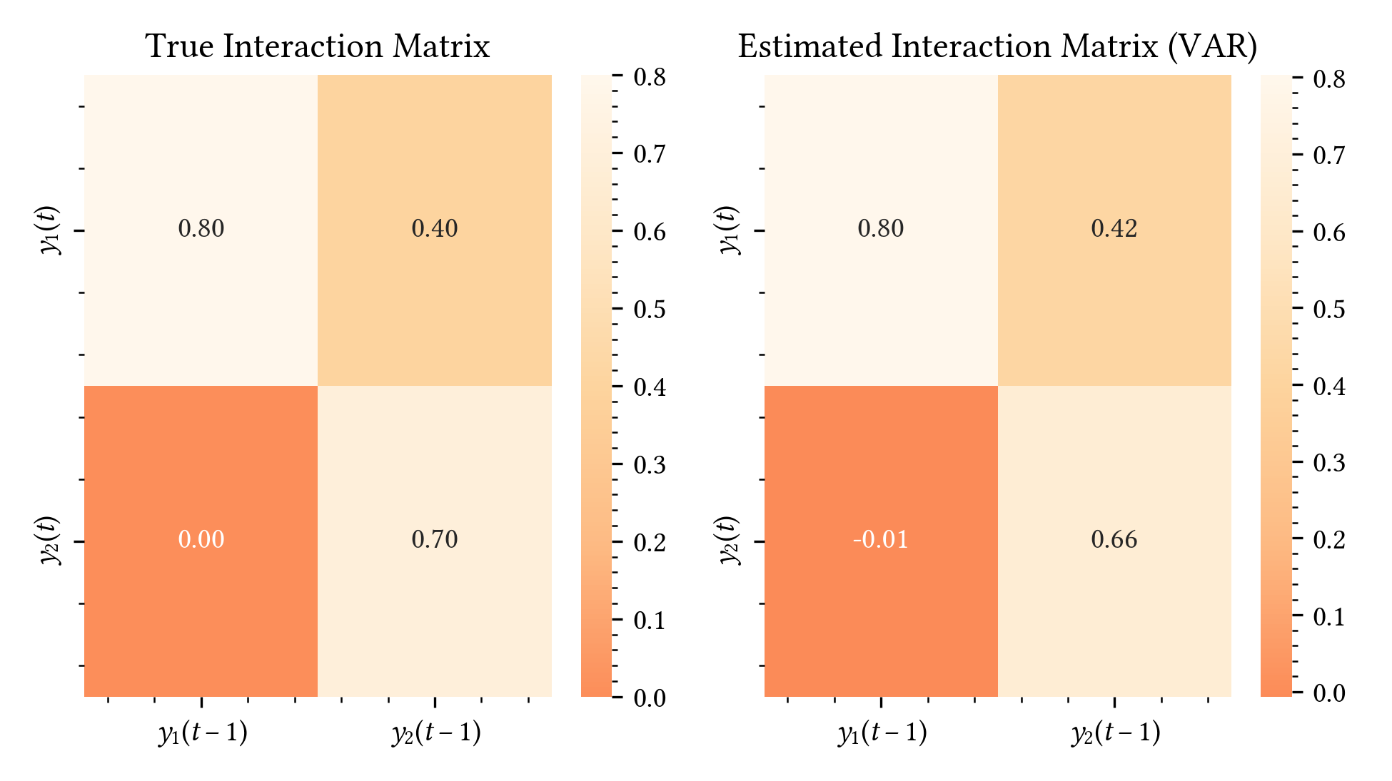
Visualizing process coupling

  • Heatmap: Visualizes coefficient matrix \mathbf{A}.
  • Interpretation:
    • Off-diagonal color \to Interaction strength.
    • Zero \to Decoupled.
  • Reveals network structure (one-way vs two-way).
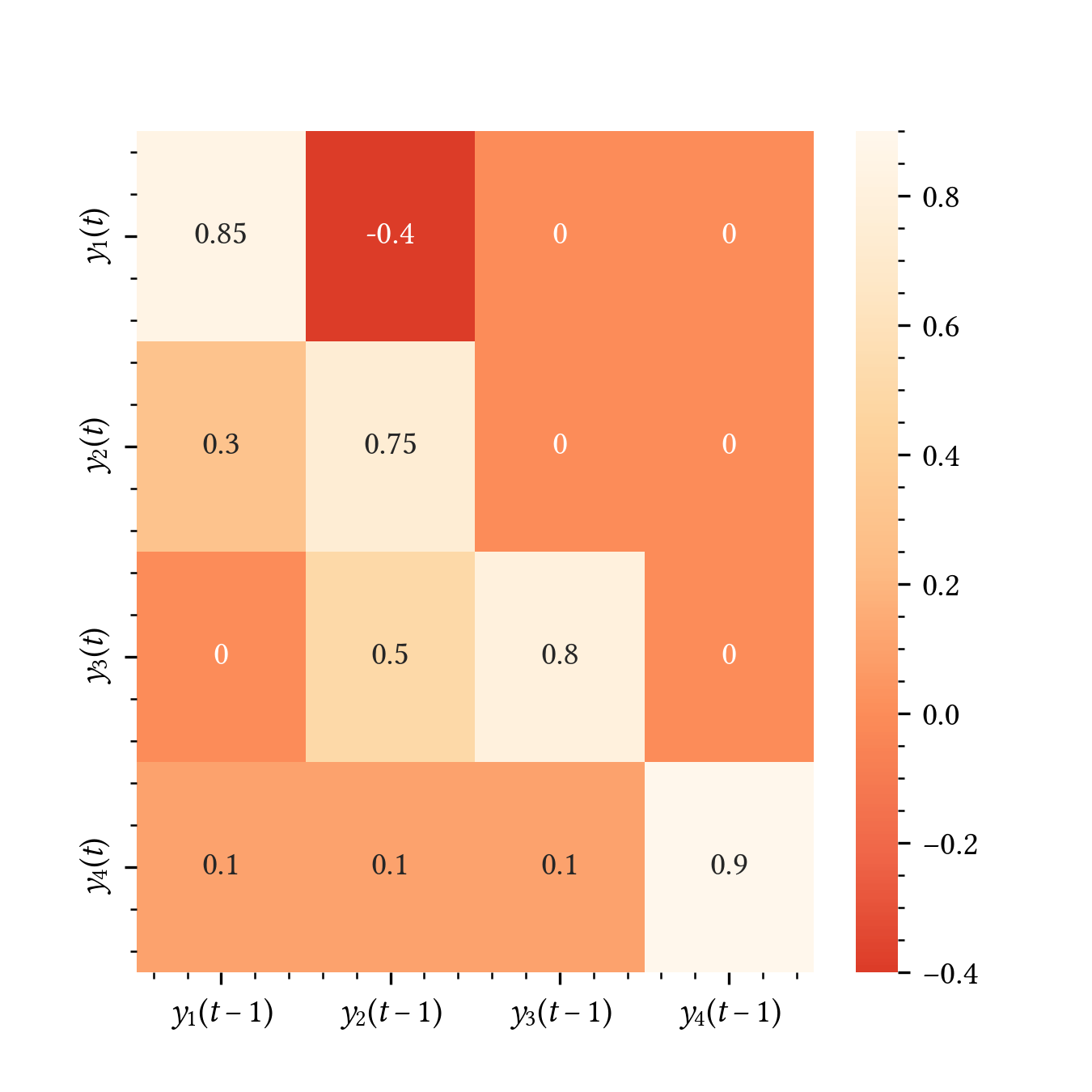
Example: Identifying topology from data

  • Scenario: 2-variable one-way interaction (y_2 \to y_1).
  • Goal: Recover structure from data alone (no physics).
  • Method: Fit Vector Autoregressive (VAR) model.
    • Inspect off-diagonal coefficients.
  • Result:
    • y_2 \to y_1 coefficient is significant.
    • y_1 \to y_2 coefficient is zero.
    • Topology successfully identified.

Granger Causality

  • Definition: Variable X “Granger-causes” Y if past X improves prediction of Y beyond past Y alone.
  • Test: Compare two models.
    1. Restricted: Uses only Y history.
    2. Unrestricted: Uses both X and Y history. y(t) = c + \sum a_i y(t-i) + \sum b_j x(t-j) + e(t)
  • Hypothesis: H_0: b_j = 0 (Null: No causality).
    • Reject if p-value < 0.05.

Defining model order (AIC)

  • Challenge: How many lags (p) to include?
    • Too few: Misses dynamics.
    • Too many: Overfitting/noise.
  • Akaike Information Criterion (AIC): \text{AIC} = 2k - 2\ln(\hat{L})
    • Penalizes complexity (k) vs. fit (\hat{L}).
  • Goal: Minimal AIC \to Optimal lag order.

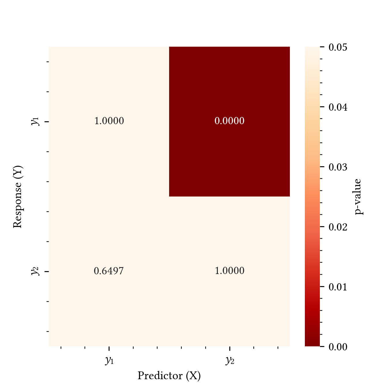
Granger Causality Matrix

  • Heatmap of p-values.
  • Interpretation:
    • Low p-value (< 0.05): Causal link.
    • High p-value: Coincidence.
  • Example:
    • y_2 \to y_1 (p < 0.05): Confirmed coupling.
    • y_1 \to y_2 (p \approx 1.0): No feedback.
  • Distinguishes physical coupling from correlation.
Limits of dynamic measurement

Temporal fidelity

  • Problem: Process is continuous; data is discrete.
    • Discrete measurements must preserve spatial/temporal content.
  • Critical factors:
    1. Sampling frequency (Aliasing).
    2. Signal-to-noise ratio (Observability).
    3. Compression (Historian artifacts).
    4. Resolution (Quantization).
    5. Sensor dynamics (Lag).
  • Rule: Information lost here cannot be recovered by modeling.

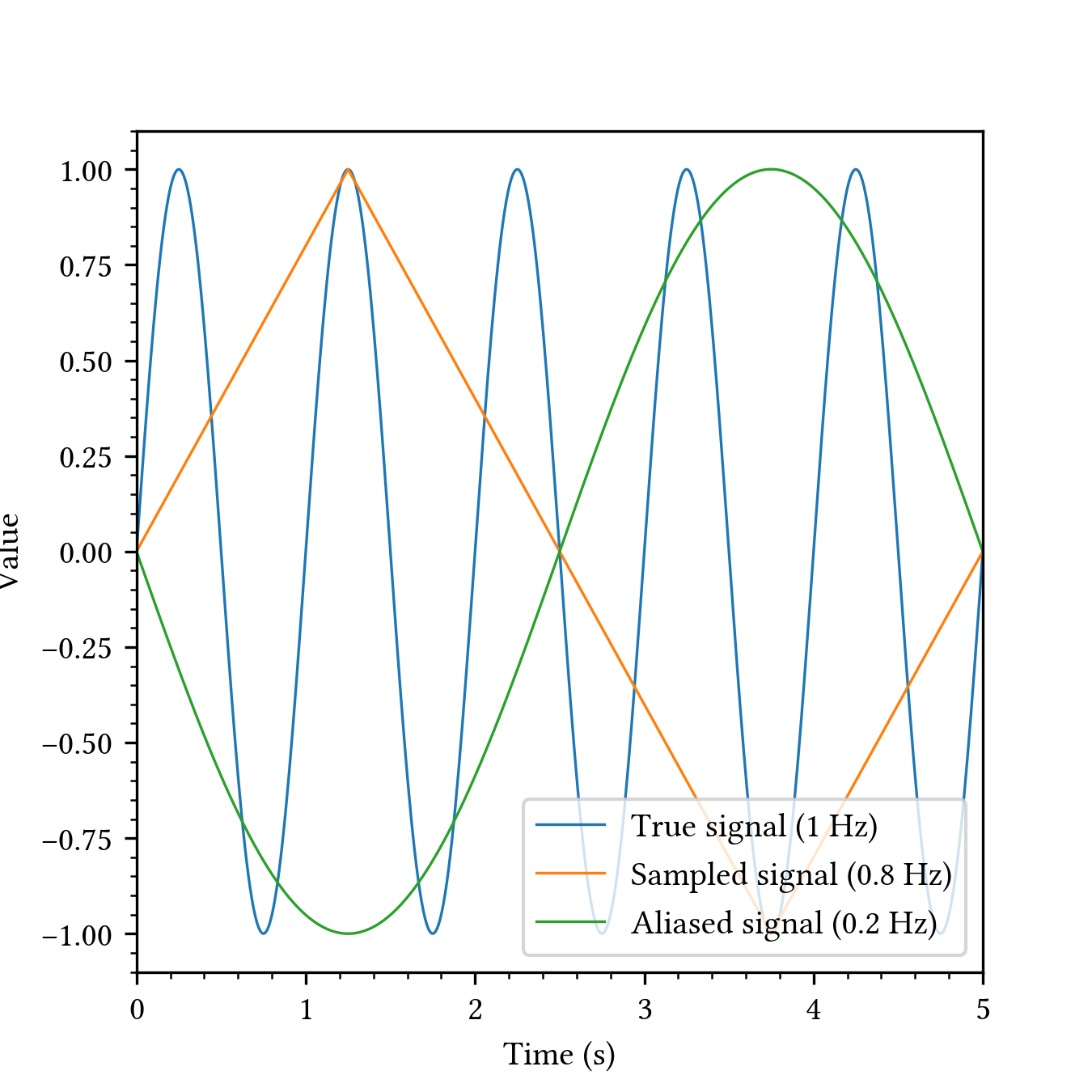
Sampling frequency & Aliasing

  • Nyquist Theorem: Sample at least 2x max frequency.
  • Rule of thumb: 5-10 \times faster than dominant time constant \tau.
  • Aliasing: Slow sampling creates fake low-freq trends.
    • Example: 1 Hz sine sampled at 0.8 Hz appears as 0.2 Hz wave.
  • Danger: Controller fights phantom dynamics.
Signal-to-noise ratio (SNR)

  • SNR: Ratio of signal power to noise power. \text{SNR} = \frac{\sigma^2_{\text{signal}}}{\sigma^2_{\text{noise}}} \approx \frac{\sigma^2_{\text{total}} - \sigma^2_{\text{noise}}}{\sigma^2_{\text{noise}}}
  • Decibels (dB): \text{SNR}_{\text{dB}} = 10 \log_{10}(\text{SNR}).
  • Impact: Low SNR \to High uncertainty in \tau, K estimates.

SNR Estimation Example

  • CSTR Data:
    • Noise variance (steady region): \sigma^2 \approx 9.6.
    • Total variance (dynamic region): \sigma^2 \approx 12.5.
    • SNR \approx 1.29 (12.9 dB).
  • Rule of Thumb: Desired SNR > 10 (10 dB) for identification.
  • Conclusion: High noise requires pre-filtering.

Data compression (Historians)

  • Swinging Door algorithm:
    • Saves point only if it deviates from slope (E_{dev}).
    • Reduces storage by 90%+.
  • Artifacts:
    • Destroys high-frequency content (noise).
    • Data looks like piecewise linear segments.
  • Advice: Request raw/interpolated data; beware “straight lines”.

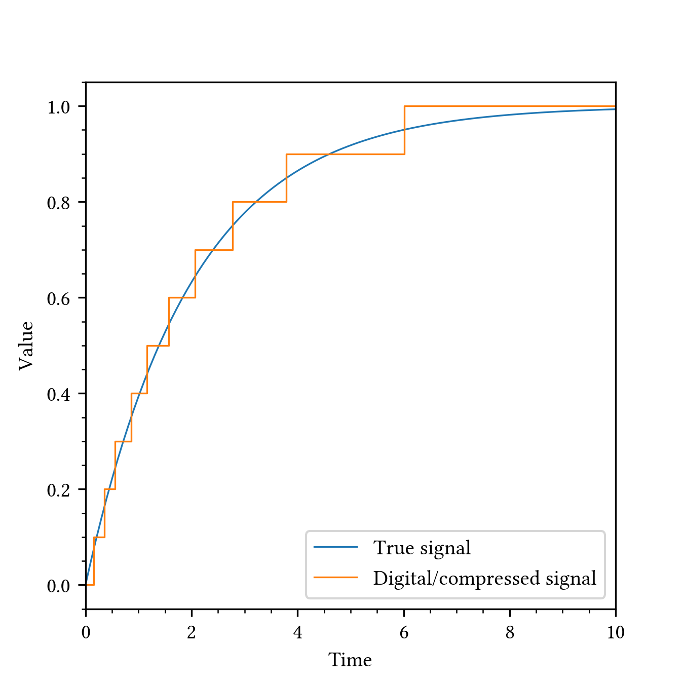
ADC Resolution & Quantization

  • Cause: Low bit depth or aggressive compression.
  • Effect: Smooth signals turn into steps.
    • Derivative dy/dt becomes series of infinite spikes.
  • Mitigation:
    • Low-pass / Savitzky-Golay filtering.
    • Kalman filtering (treat as measurement noise).
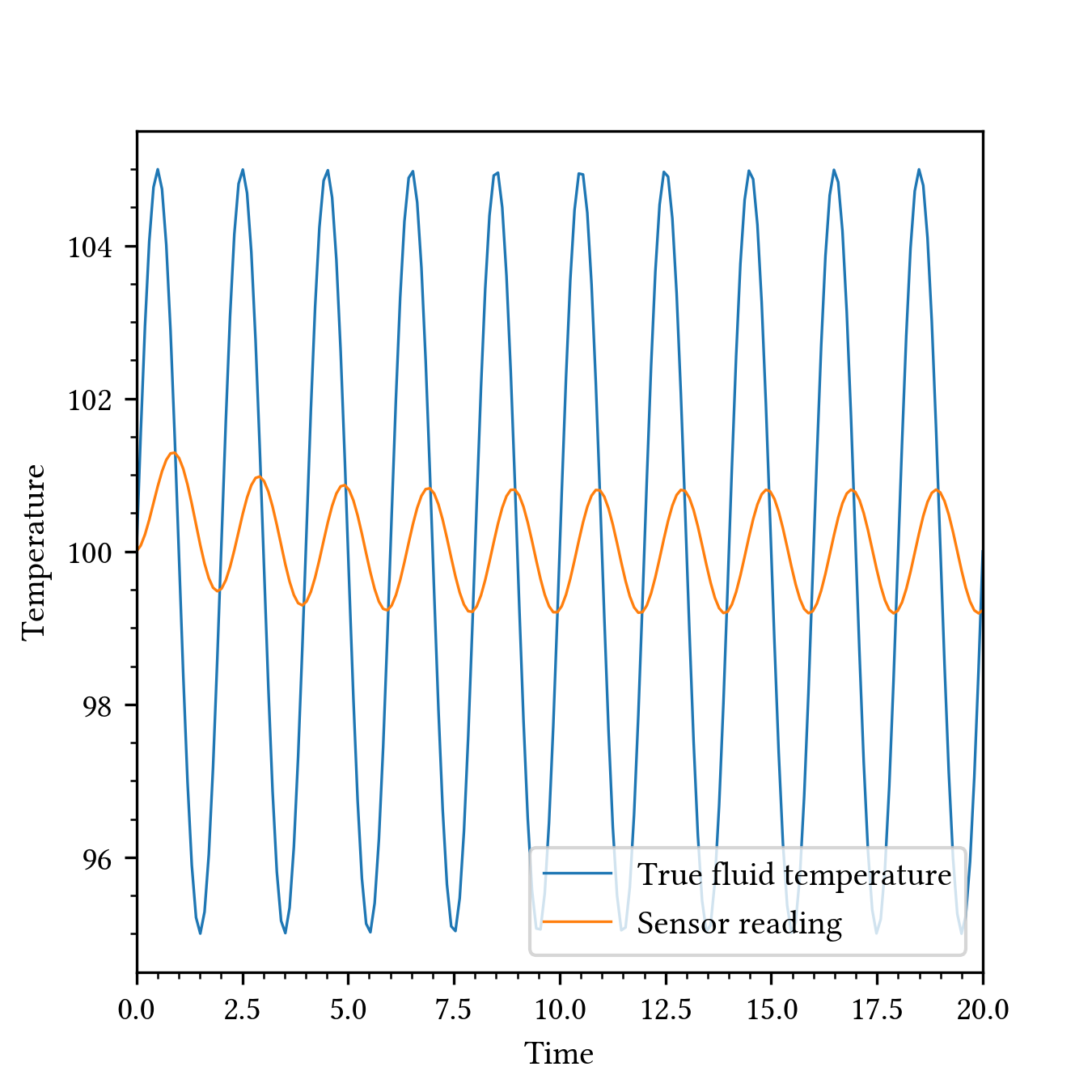
Measurement lag (Sensor dynamics)

  • Reality: Sensors have their own dynamics (e.g., thermowells).
    • Acts as a low-pass filter.
  • Consequence:
    • Process appears slower/more stable than reality.
    • Underestimates variability.
  • Risk: Controller designed too slow for real disturbances.
Recap

  • Exploratory Analysis: Visualization (Scatter/Parallel plots) distinguishes operating regimes from sensor artifacts.
  • Data Health: Robust pre-processing (Hampel filtering) and Reconciliation (Physics-based balances) provide the data foundation.
  • Steady-State: Automated detection (Rolling std + Slope) enables robust gain estimation and model initialization.
  • Dynamic Structure: ARX/ARMAX models capture process inertia (\phi), oscillations (AR2), and dead-time.
  • Causal Mapping: VAR models and Granger Causality recover the interaction topology from multi-variable signatures.
  • Information Ceiling: Sampling rates (Aliasing), SNR, and sensor lags define the upper limit of model fidelity.

Discussion Question

If our process data is already limited by noise, delays, or slow sampling, when does making a model more “sophisticated” actually start making our control worse? How do we know when to stop adding more complexity?

Data for hands on exercises