Latent Variable Methods

Data to Dynamics

Table of contents

• Process data environment
• Principal component analysis
• Case study: Portland cement data
• Process modeling using PCA
• Fault Identification and Diagnosis

Process data environment

Process data environment

• Densely instrumented environments
  • ~5,000 to 50,000+ tags (sensors) per plant
• Generate massive high-frequency data
  • Sampling rates: 1 Hz to 100 Hz
  • Gigabytes of historized data daily
• DCS (Distributed Control System)
  • Digital brain of the plant recording historical data
• DCS Role:
  • Record thousands of variables
  • Temperatures, pressures, flow rates, compositions
  • Tank levels, valve positions, motor speeds
  • Power consumption, vibrations, pH/conductivity

High-dimensional vs. Low-dimensional space

• What is Dimension?
  • In data science: 1 variable = 1 dimension
  • 1,000 sensors create a 1,000-dimensional database
  • Each timestamp records a single “point” in this space
• Actual degrees of freedom are remarkably small
  • Minimum independent variables to define system state
  • Independent “knobs” vs. dependent sensors
  • 1000s of signals tied by physical laws
    • Mass balance: In - Out = Accumulation
    • Phase equilibrium: T and P locked together
    • Stoichiometry: Chemicals change in fixed ratios
  • Only few variables can change independently

High-dimensional vs. Low-dimensional space

• Underlying physics exist in lower-dimensional space
  • 100 sensors = 100-dimensional space
  • Physical constraints restrict data variation
  • Data points follow rigid physical patterns
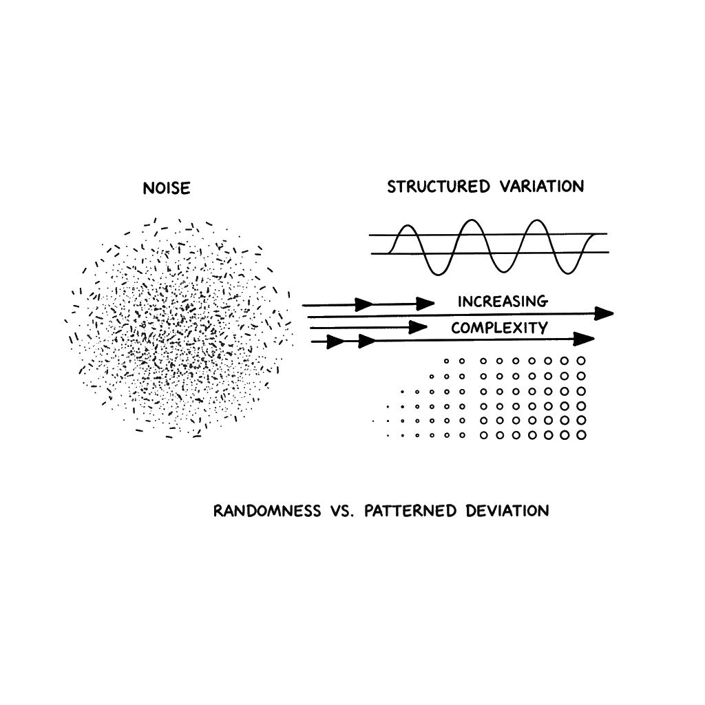
  • Measurements don’t vary randomly in all directions
  • Sensors fluctuate in sync when driven by the same physical event
  • This shared behavior represents the real state of the process

Discrepancy in sensor systems

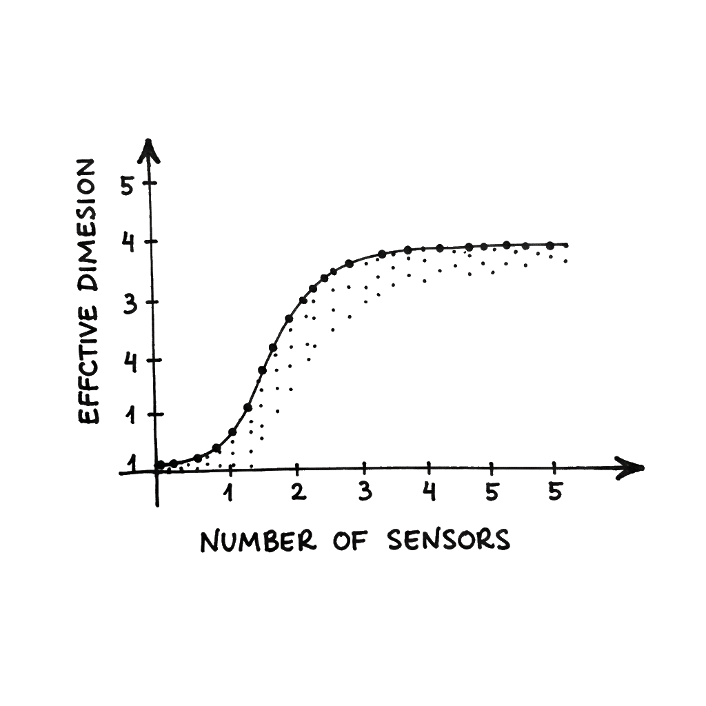
• Discrepancy between sensor count and system dynamics
• Sensors added for safety and local control
• System dynamics driven by few phenomena
  • Reaction rate change: affects T, P, and all conc.
  • Main feed disturbance: ripples through every equipment downstream

Information sparsity and redundancy

• Gap between measurement count and dynamic events
  • 10,000 sensors \neq 10,000 independent pieces of information
  • Information is sparse relative to the raw data volume
  • Redundancy is the mathematical bridge across this gap
• Redundant signals capture shared information

Nature of latent variables

• Latent variables inherently manifest in process data
  • Latent: “Hidden” or unobserved factors
  • Drivers that cannot be measured directly
  • Mathematically inferred from correlated physical sensors
• True driving forces often unobservable
• Hidden factors buried within sensor data
• Extracted mathematically from correlations
• Separate underlying signal from measurement noise
• Factors represent physical “reality” of the process

Physical constraints and latent variables

• Conservation laws (Mass, energy, momentum)
  • Impose strict algebraic constraints
  • Link flows, levels, and pressures mathematically
• Thermodynamics (Phase equilibria)
  • Links temperature, pressure, and composition
  • Restricts independent variable movement (Collinearity)

Operational impacts on data structure

• Feedback control (PID loops)
  • Locks inputs and outputs into correlated trajectories
  • Masks open-loop dynamics to reach setpoints
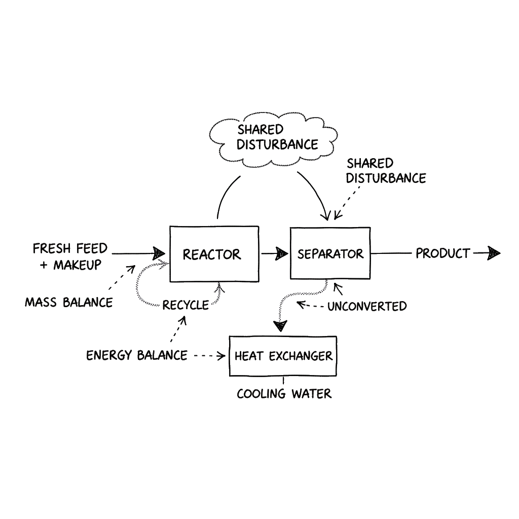
• Process topology (Recycle loops)
  • Shared disturbances propagate through networks
  • Causes distant measurements to fluctuate in sync
• \Rightarrow Physics and control force sensor data to follow synchronized patterns

Ordinary least squares regression

• OLS (Ordinary Least Squares)
  • Standard linear regression method
  • Minimizes squared distances to the data points
  • Assumption: Observed variables are independent

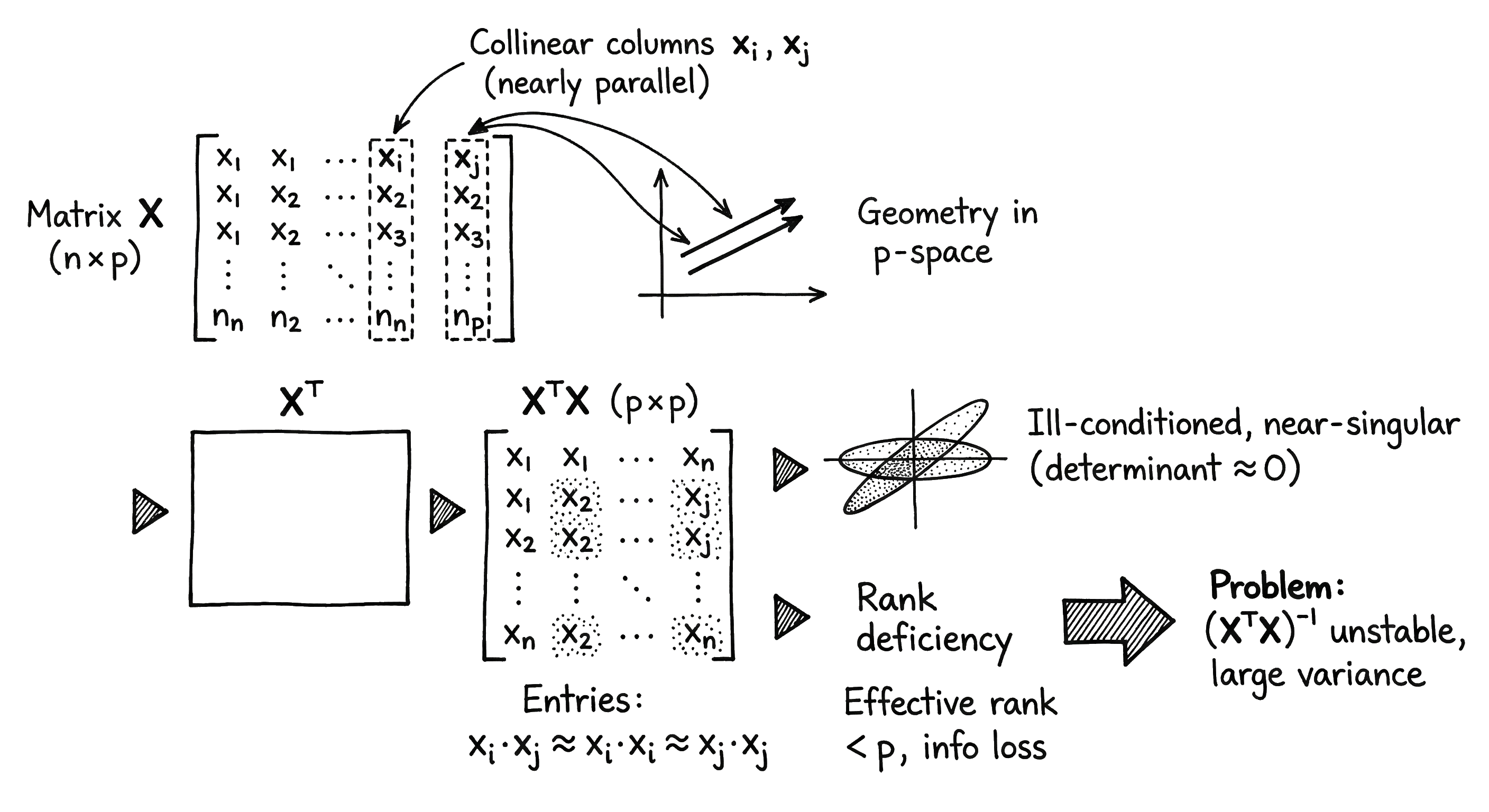
Mathematical failure on redundant data

• Failure on redundant data:
  • Covariance matrix (X^\top X) becomes ill-conditioned
    • Summarizes how all variables fluctuate together
    • OLS requires inverting this matrix to find weights
    • Redundant data \approx dividing by zero during inversion
  • High correlation makes matrix inversion unstable
  • Leads to explosive variance in model results
• Resulting models are physically meaningless

Data projection and latent factors

• Projects correlated sensor data onto latent variables
• Extracts the shared signal driving synchronized fluctuations
• Defines a lower-dimensional subspace that captures process state
• Separates structured fluctuations from random measurement noise
• Ensures numerical stability by creating uncorrelated factors

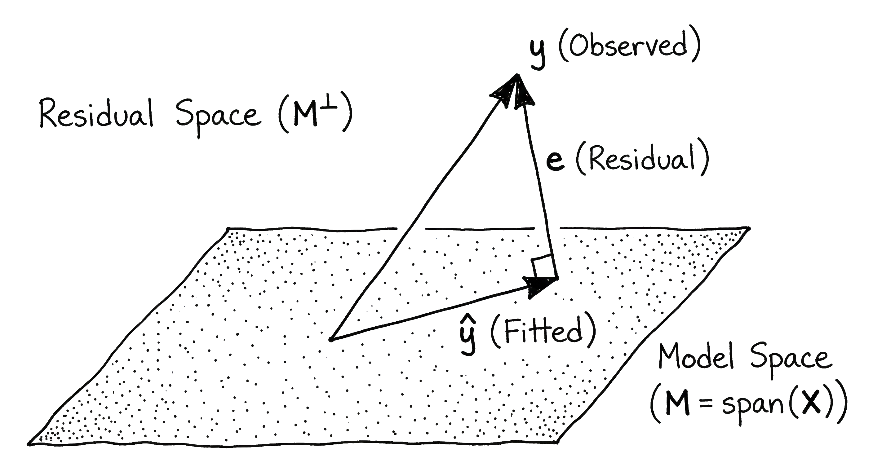
Example 1: Distillation mass balances

• Measured: Feed, distillate, and bottoms (flows + compositions)
• 6 sensors \neq 6 degrees of freedom
• Rigidly tied by overall and component mass balances
• If feed rate increases, D and B must rise to maintain balance
• Variation is restricted: 6 numbers move like they are only 2
• Throughput: The primary latent factor driving all 6 sensors

Example 2: Heat exchanger energy balances

• Measured: 4 Temperatures (in/out) + 2 Flow rates
• 6 sensors \neq 6 degrees of freedom
• Hot side energy loss = Cold side energy gain
• All 6 measurements are mathematically “locked” by one equation
• State can be summarized by 1-2 latent factors
• Heat load (Q): The latent factor representing energy exchange

Example 3: Reactor-separator recycle loops

• Measured: Dozens of sensors across reactor, separator, and recycle line
• 20+ sensors \neq 20+ degrees of freedom
• Disturbance in feed cycles back through the recycle line
• Creates a plant-wide “ripple” across distant units
• All sensors show synchronized fluctuations over time
• Recycle intensity: The latent factor capturing loop-wide behavior

Example 4: Distillation thermal profiles

• puritiy monitored by dozens of tray thermocouples
• Temperatures follow bubble-point curves
• Adjacent tray temperatures move identically
• 50 trays \neq 50 degrees of freedom
• Profile described by 2-3 latent factors:
  • Average position, slope, and inflection point

Principal component analysis

Principal component analysis

• Exploratory technique for dimensionality reduction (2D or 3D)
• Key capabilities:
  • Simplify data: Minimize variables while maintaining information
  • Identify outliers: Detect abnormal process behavior
  • Find patterns: Reveal hidden relationships in high-dimensional data
  • Visualize: Project complex datasets into viewable space
• Applications: Process monitoring, Environmental analysis, Quality control

What are Principal Components?

• Transforms high-dimensional data into new axes
• Principal Components (PCs) are linear combinations of original variables
• Ordered by explained variance:
  • PC1: Captures the greatest data spread (maximum information)
  • PC2: Orthogonal to PC1, captures next highest variance
• Each PC is uncorrelated with the others

PCA model decomposition

• Decomposes data matrix \mathbf{X} (m \times n):
  • \mathbf{X} = \mathbf{T}\mathbf{P}^\top + \mathbf{E}
• Scores (\mathbf{T}): Observation coordinates in reduced space
• Loadings (\mathbf{P}): Coefficients defining the PCs
• Residuals (\mathbf{E}): Unexplained noise/error

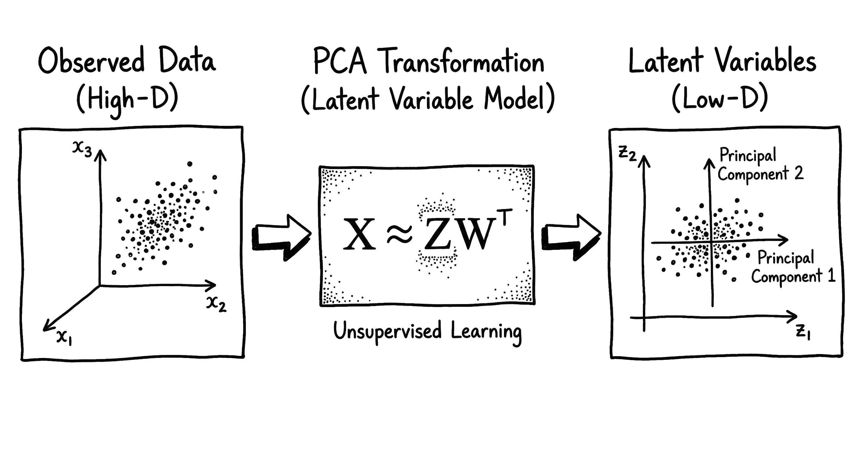
Visualizing variance

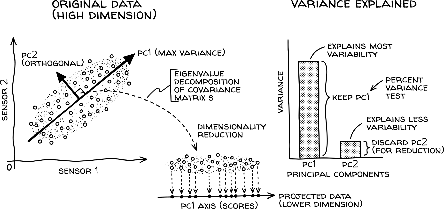
• PCs show directions of maximal variance
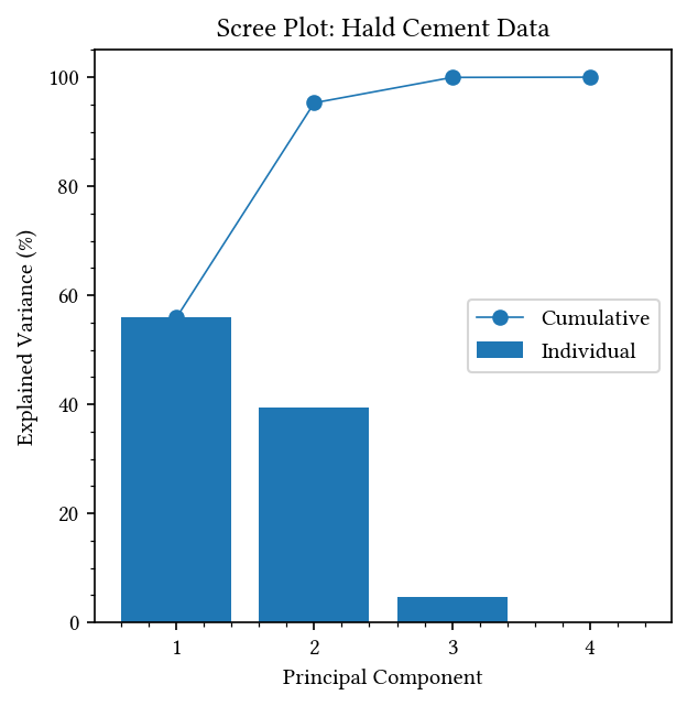
• Scree plot shows info retained per component
• First few PCs often capture >90% of variability
• Residuals represent the distance “off” the model plane

Case study: Portland cement data

The Hald dataset

• 4 Ingredients (% weight):
  • C3A: Tricalcium aluminate
  • C3S: Tricalcium silicate
  • C4AF: Tetracalcium aluminoferrite
  • C2S: Dicalcium silicate

• Heat (cal/gm): response variable
• Evolution after 180 days of hardening
• Source: Woods et al. (1932)
• Classical example of multi-collinearity

Redundancy in cement composition

• 4 ingredients \neq 4 degrees of freedom
• Chemical constraint: \sum \text{Ingredients} \approx 100\%
• If three ingredients are known, the fourth is nearly fixed
• This created a rank-deficient system
• OLS regression coefficients become unstable and meaningless
• PCA solution: Identifies the 2-3 independent “mixtures”

Correlation structure

• Strong correlations confirm redundancy:
• Matrix:

	C3A	C3S	C4AF	C2S
C3A	1.00	0.23	-0.82	-0.25
C3S	0.23	1.00	-0.14	-0.97
C4AF	-0.82	-0.14	1.00	0.03
C2S	-0.25	-0.97	0.03	1.00

• C3S vs C2S (r = -0.97): Nearly perfect inverse relationship
• C3A vs C4AF (r = -0.82): Strong inverse relationship
• These are the physical constraints visible in data

Variance capture

• Scree Plot: Variance captured per component
• PC1: Dominant direction (~95%)
• PC2: Secondary orthogonal direction (~4%)
• Result: 2 components capture >99% of valid information
• Remaining components are noise

Biplot analysis

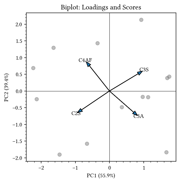
• Biplot: Overlays scores and loadings
• Scores: Observation relationships
• Loadings: Variable correlations
• Variables pointing in opposite direction are negatively correlated
  • C3S vs C2S (Opposite)
  • C3A vs C4AF (Opposite)

Process modeling using PCA

Process modeling using PCA

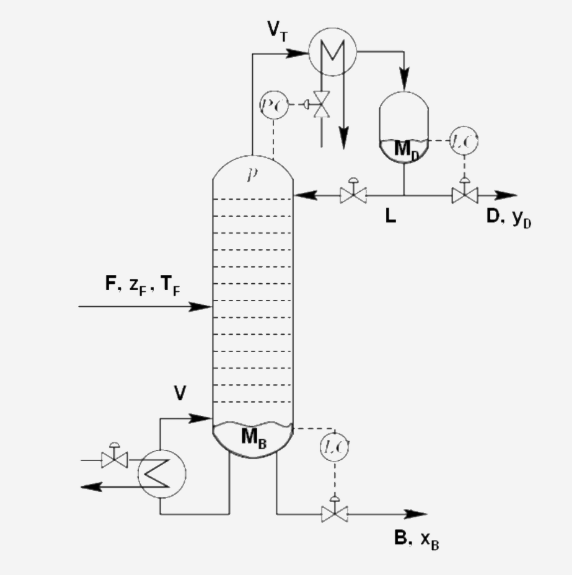
• Distillation column example
  • Separating Methanol – Ethanol mixture
  • CVs: Y_D (Distillate), X_B (Bottoms)
  • MVs: D, B, L, V
  • DVs: F, T, z
• Workflow:
  • Phase I: Model steady state with PCA
  • Phase II: Project new observations on model and detect deviation

Phase I: Model steady state with PCA

• Objective: Capture normal operating conditions (NOC)
• Reduce dimensionality while retaining information
  • 7 variables (CVs + MVs + DVs) \rightarrow highly correlated
• Model Selection:
  • Calculate limits for T^2 (Model plane) and SPE (Residuals)
  • Stop when variance explained reaches threshold (e.g., >90%)

Phase I: Model steady state with PCA

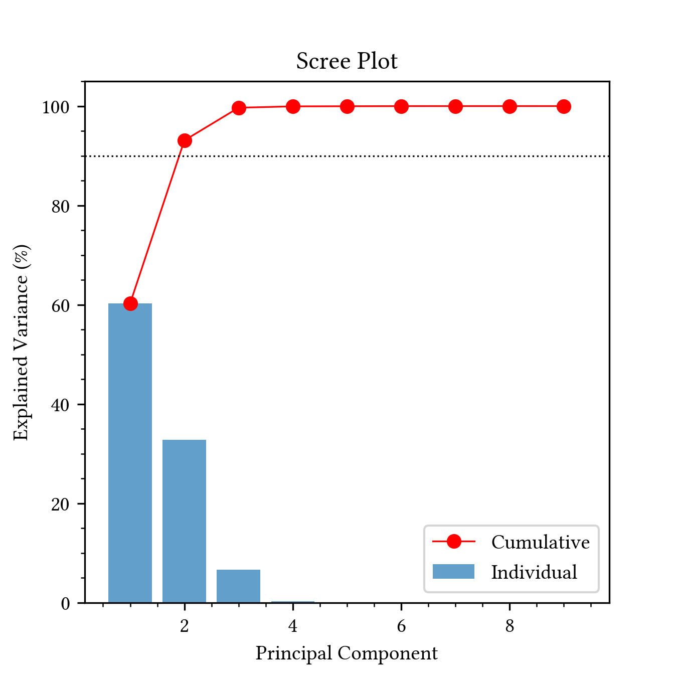
• Scree Plot Analysis
  • PC1: Dominant process direction
  • PC2: Secondary direction
  • Result:
    • 2 Components selected
    • 93.1% total variance explained
    • Remaining 5 dimensions are noise

Phase II: Project new observations

• Monitoring Strategy
  • Project new data onto defined PCA model
  • Detect deviations from “Normal” behavior
• Two key metrics:
  • SPE (Squared Prediction Error): Residuals distance off the model plane
  • T^2 (Hotelling’s T-squared): Mahalanobis distance within the model plane

Distance in correlated spaces

• Distance measure that accounts for data correlation.
• Measures how many “standard deviations” a point is from the mean.

Euclidean (Standard)

• Assumes spherical distribution.
• d = \sqrt{\sum (x_i - \mu_i)^2}
• Ignores interaction between variables.

Mahalanobis (T^2)

• Accounts for elliptical shape.
• T^2 = (\mathbf{x}-\mathbf{\mu})^\top \mathbf{\Sigma}^{-1} (\mathbf{x}-\mathbf{\mu})
• Scale-invariant and correlation-aware.

• In PCA: T^2 is the Mahalanobis distance in the model plane.

Phase II: Monitoring Metrics

Hotelling’s T^2 Statistic

• Mahalanobis distance in the score space (model plane).
• Detects extreme deviations consistent with the correlation structure.
• Equation: T^2 = \sum_{a=1}^{A} \frac{t_a^2}{\lambda_a} = \mathbf{x}^\top \mathbf{P} \mathbf{\Lambda}^{-1} \mathbf{P}^\top \mathbf{x}
  • t_a: Score on PC a
  • \lambda_a: Eigenvalue (variance) of PC a

Squared Prediction Error (SPE)

• Euclidean distance in the residual space (off model plane).
• Detects breakdown of the correlation structure.
• Equation: SPE = \sum_{j=1}^{m} (x_j - \hat{x}_j)^2 = \|\mathbf{e}\|^2
  • \mathbf{e} = \mathbf{x} - \hat{\mathbf{x}}: Residual vector
  • \hat{\mathbf{x}} = \mathbf{T}\mathbf{P}^\top: Reconstructed vector

Phase II: Project new observations

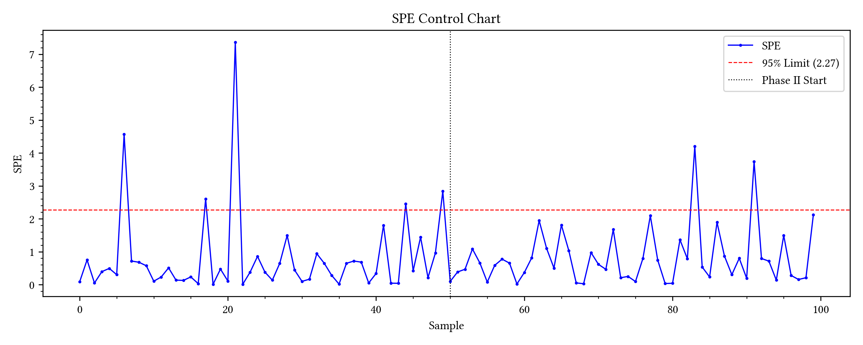
SPE control chart

• Measures distance to model
• Violation \rightarrow correlation structure broken
• Indicates new relationship or sensor fault

Hotelling’s T^2 control chart

• Measures data within NOC zone
• Violation \rightarrow extreme operating point
• Valid relationship, but unusual range

Phase II: Monitoring Results

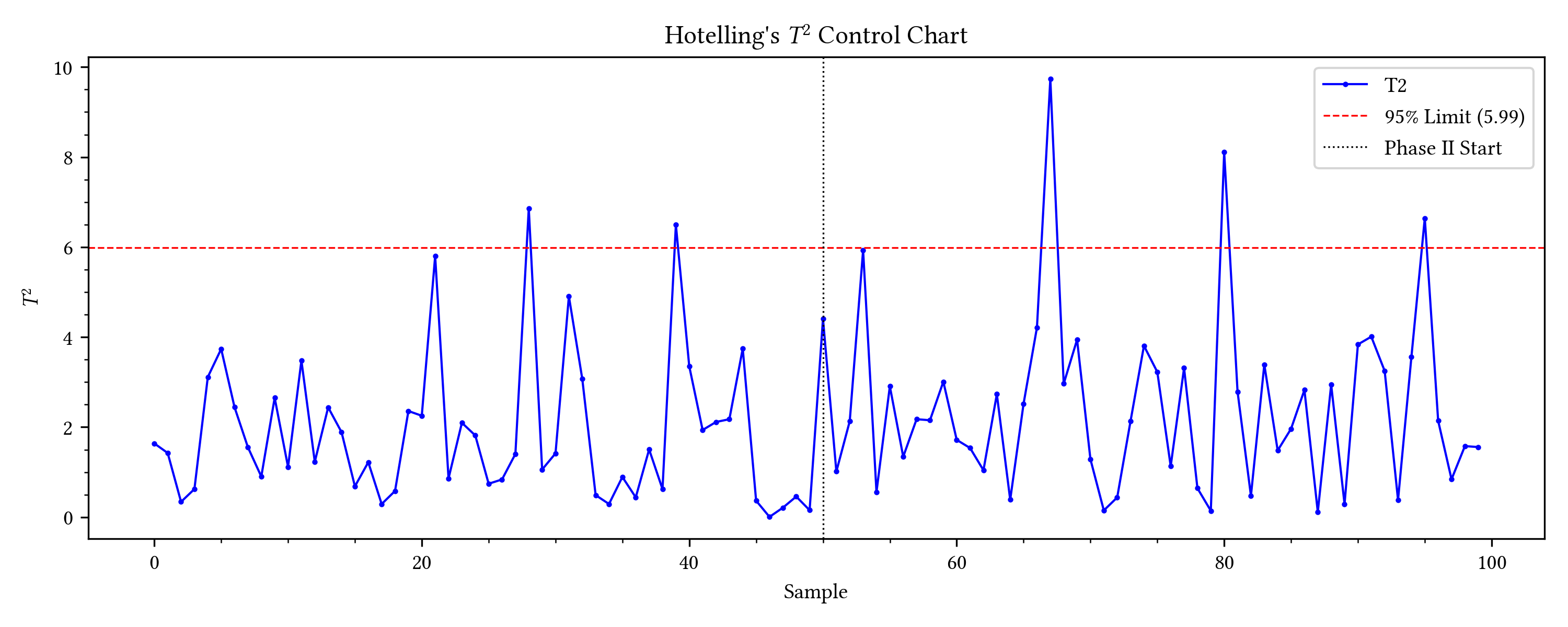
• Fault Detection:
  • Process starts in control (samples 0-50)
  • Drift introduced at sample 50
  • Both charts clearly detect the deviation
  • Exceeds 95% Confidence Limit (Red dashed line)

Fault Identification and Diagnosis

Fault Classification

• Process Disturbances:
  • Ramp: Gradual drift (e.g., fouling, catalyst decay)
  • Pulse: Temporary shift (e.g., feed quality change)
  • Spike: Sensor failure or transient shock
• Diagnosis Workflow:
  • Detect: T^2 or SPE limit violation
  • Identify: Pattern recognition (Scores)
  • Diagnose: Variable contribution (Loadings)

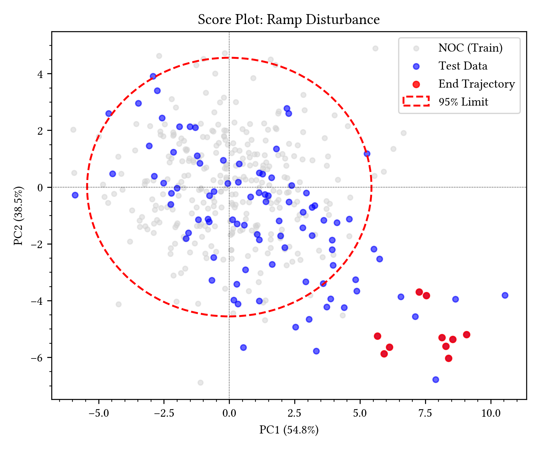
Visualizing the fault trajectory

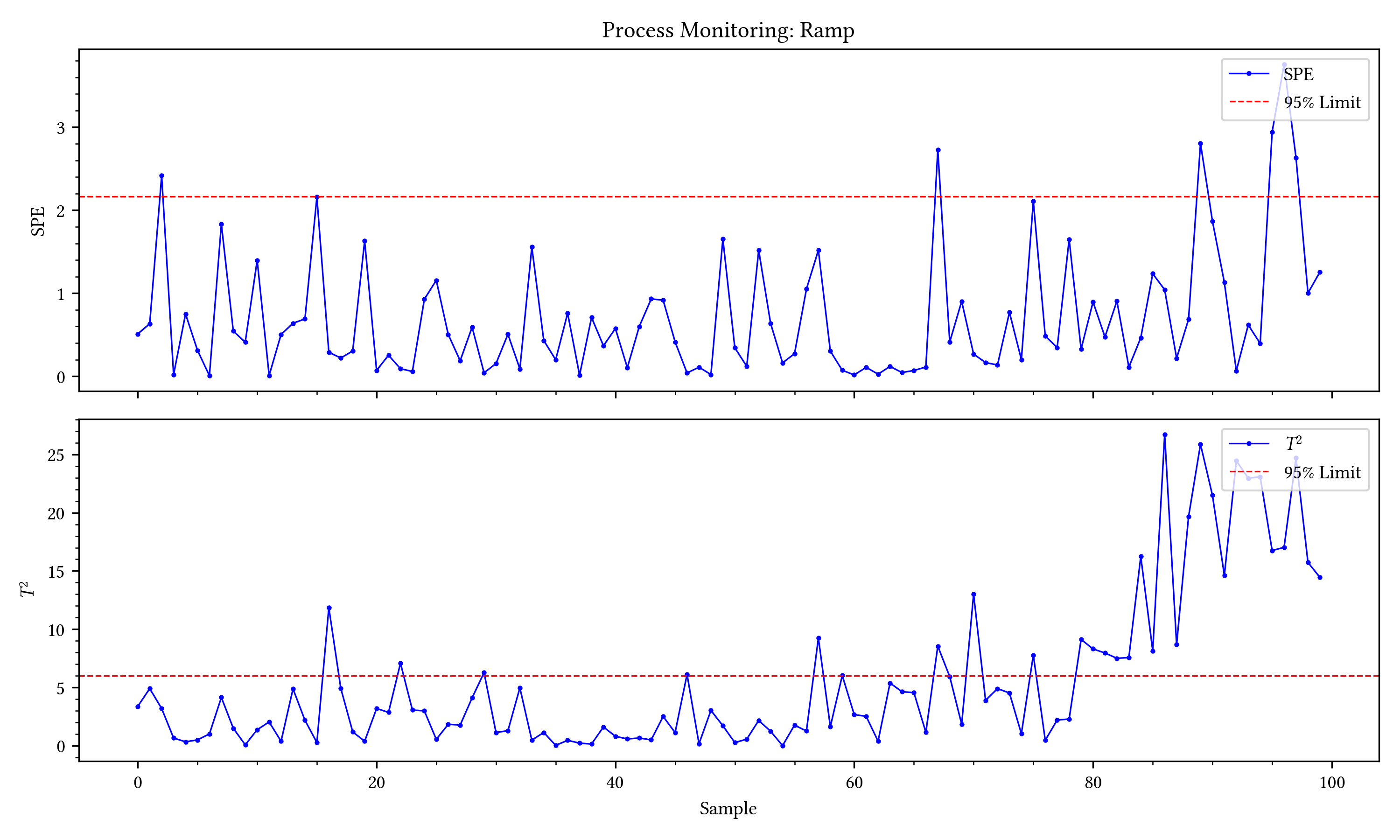
Scenario 1: Process Drift (Ramp)

Control Charts

Score Space

• Observation:
  • Slow, consistent rise in both T^2 and SPE.
  • Points move systematically away from the cluster center.
  • Insight: The process is evolving to a new state, likely due to a persistent change (e.g., heat exchanger fouling).

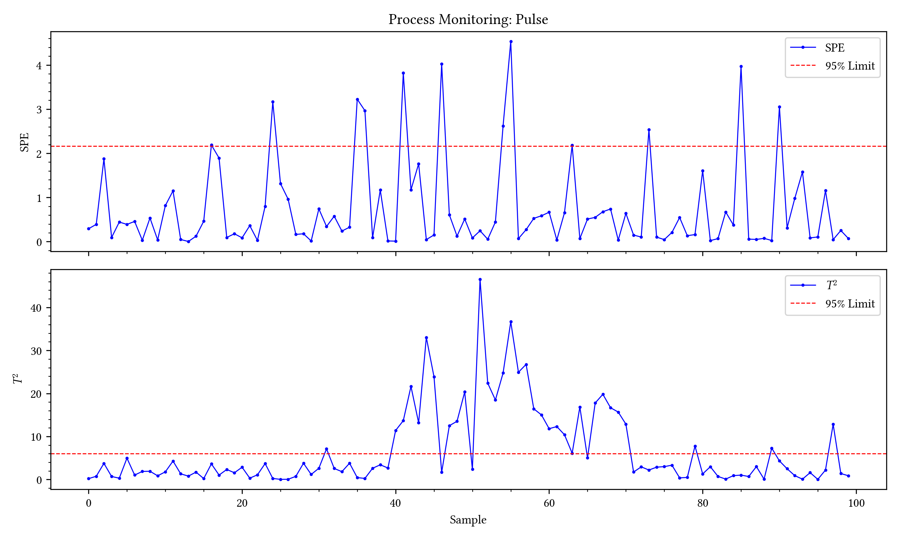
Scenario 2: Process Shift (Pulse)

Control Charts

Score Space

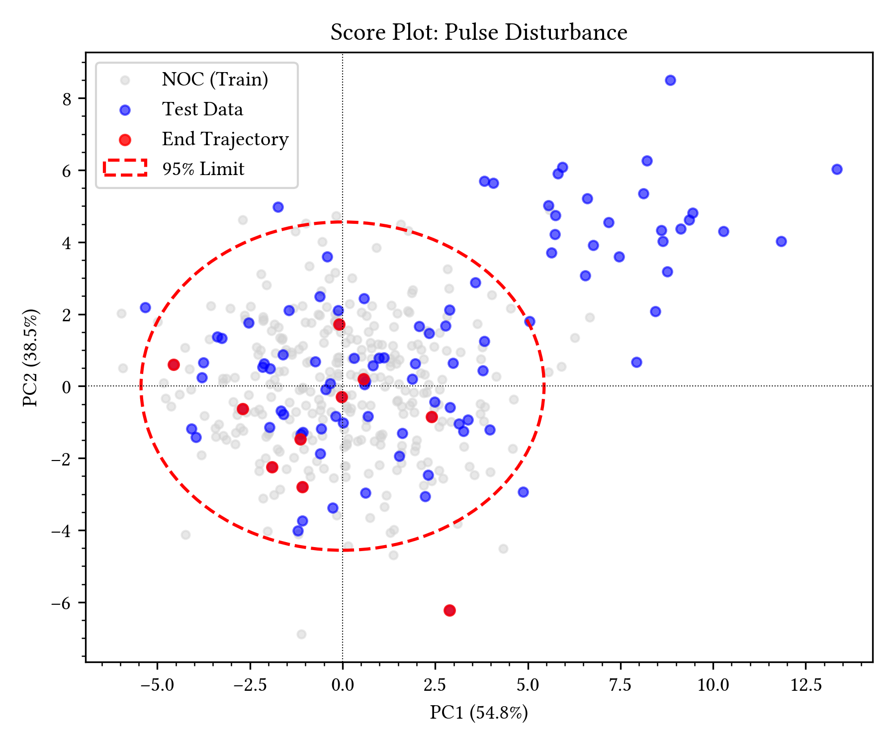
• Observation:
  • Sudden jump to a new operating region, followed by a return.
  • Points form a secondary cluster outside the 95% limit.
  • Insight: A temporary but sustained disturbance (e.g., feed composition change) moved the process to a different valid operating point (T^2 dominant).

Scenario 3: Sensor Fault (Spike)

Feature Contribution

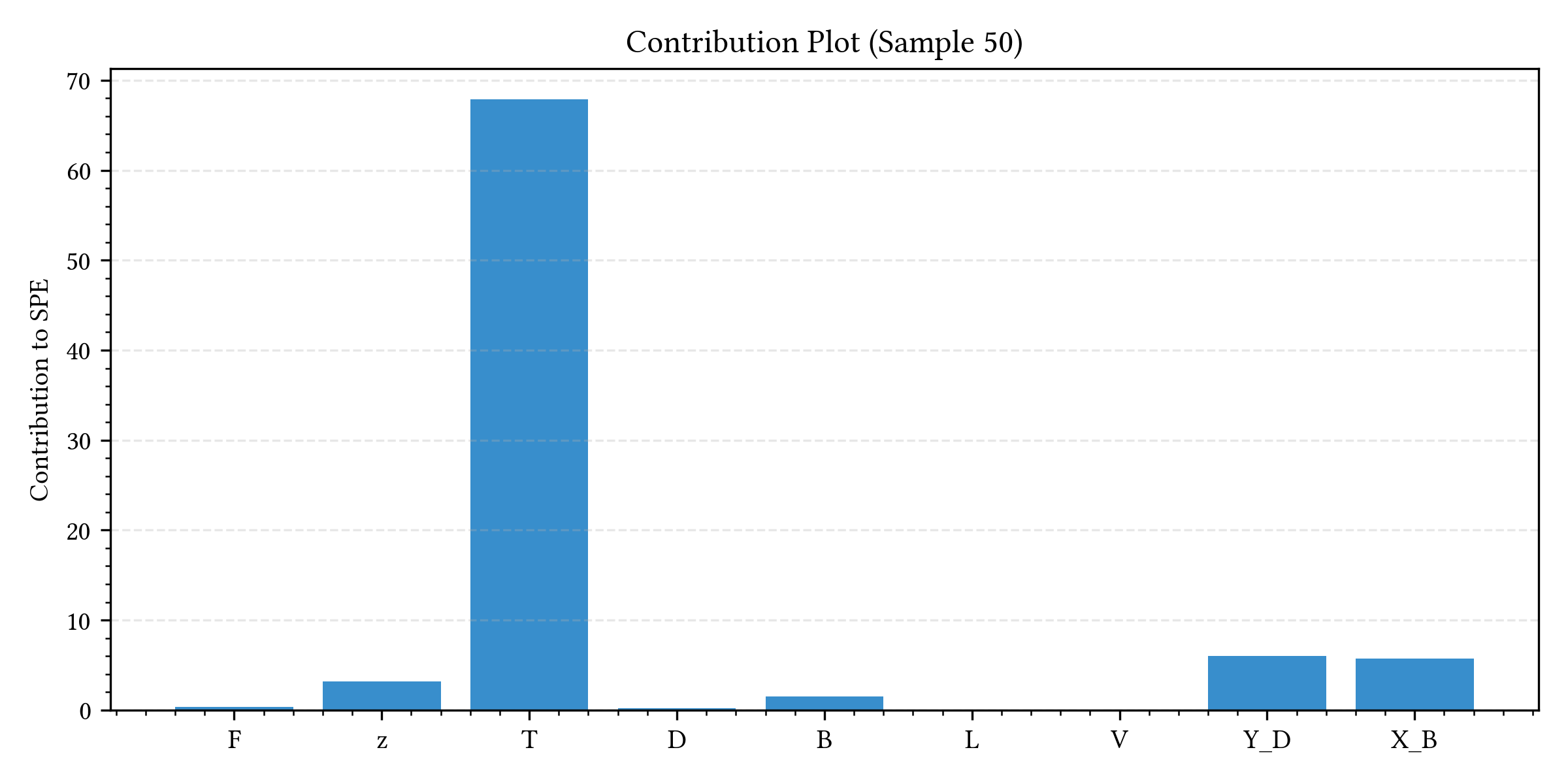
Characteristics

• Pattern:
  • Sharp, single-point violation in SPE.
  • minimal impact on T^2 (orthogonal to model plane).
• Diagnosis:
  • Contribution Plot: Decomposes the error per variable.
  • Temperature (T) shows dominant contribution.
  • Conclusion: Likely a sensor failure, not a process change.