Nonlinear and ML Models
Data to Dynamics
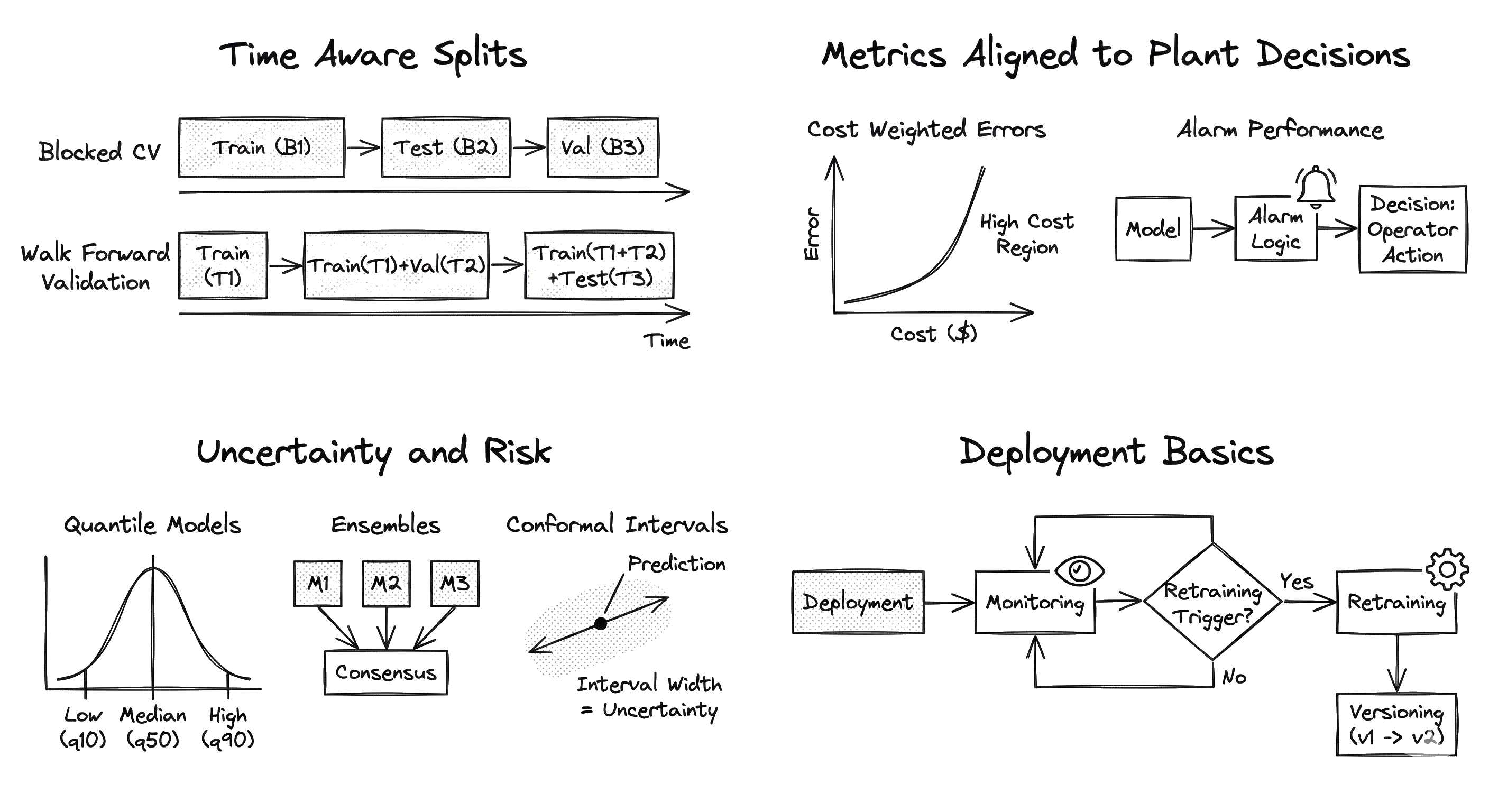
Why Linear Models Fail
- Chemical processes are inherently nonlinear
- Linear models (e.g., PCA, PLS) assume constant relationships
- Real-world complexities:
- Reaction kinetics (exponential)
- Phase transitions
- Saturation effects
- Operating regime shifts
- Relying on linear approximations can lead to poor control and monitoring performance
Machine Learning Types
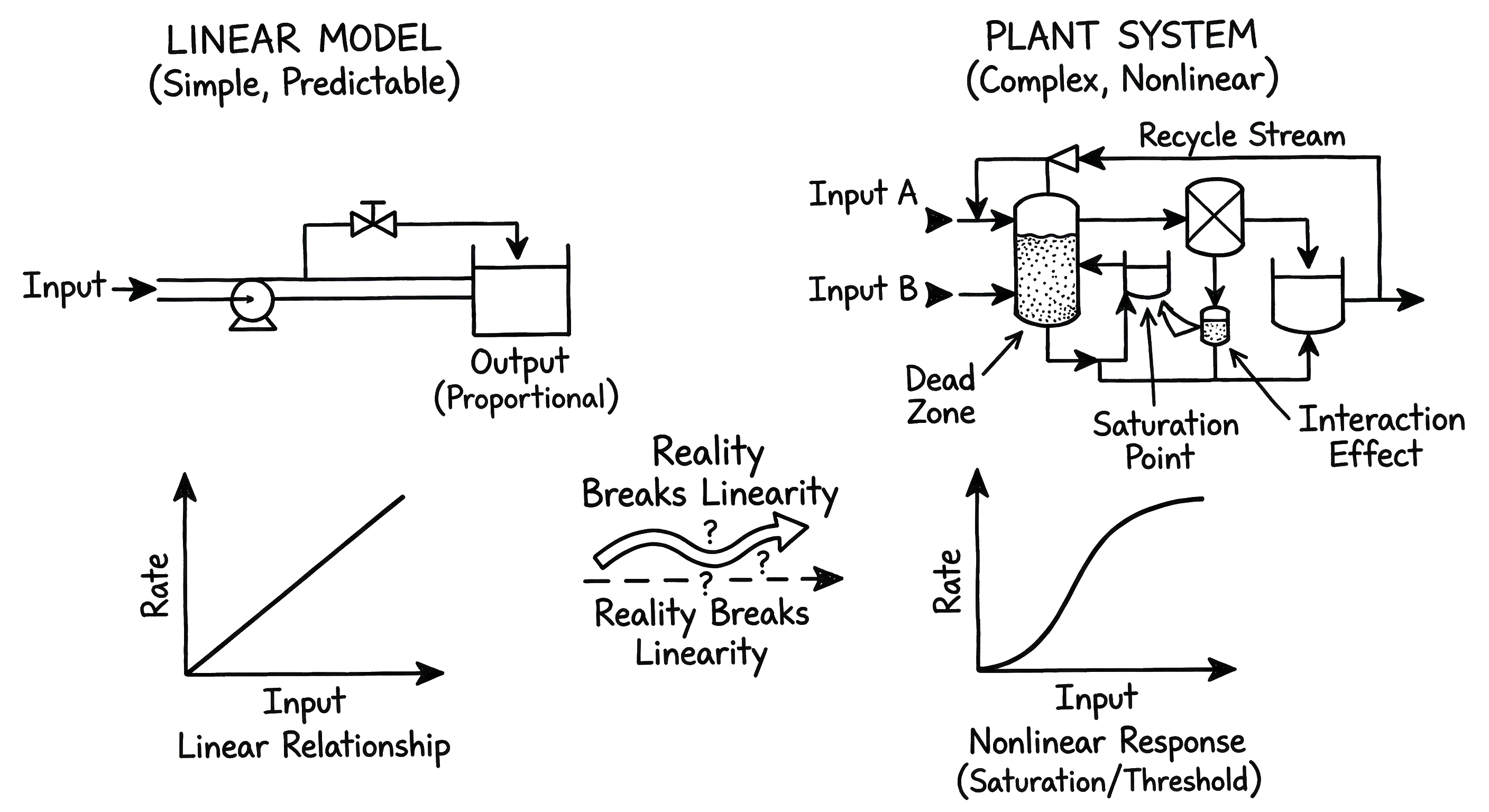
- Supervised Learning:
- Input-Output mapping
- Examples: Regression (Continuous), Classification (Discrete)
- Common for soft sensing and fault diagnosis
- Unsupervised Learning:
- Finding structure in data
- Examples: Clustering, Dimensionality Reduction
Regression Problems
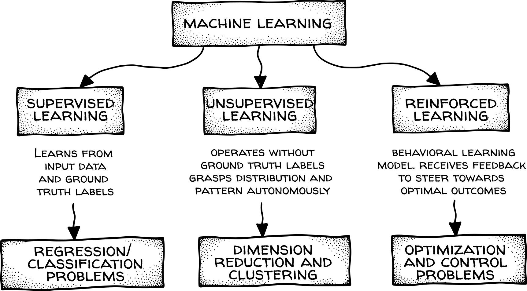
- Goal: Predict continuous process variables
- Applications:
- Product quality estimation
- Soft sensors
- Forecasting key performance indicators
- Success depends on capturing the underlying function y = f(x) accurately
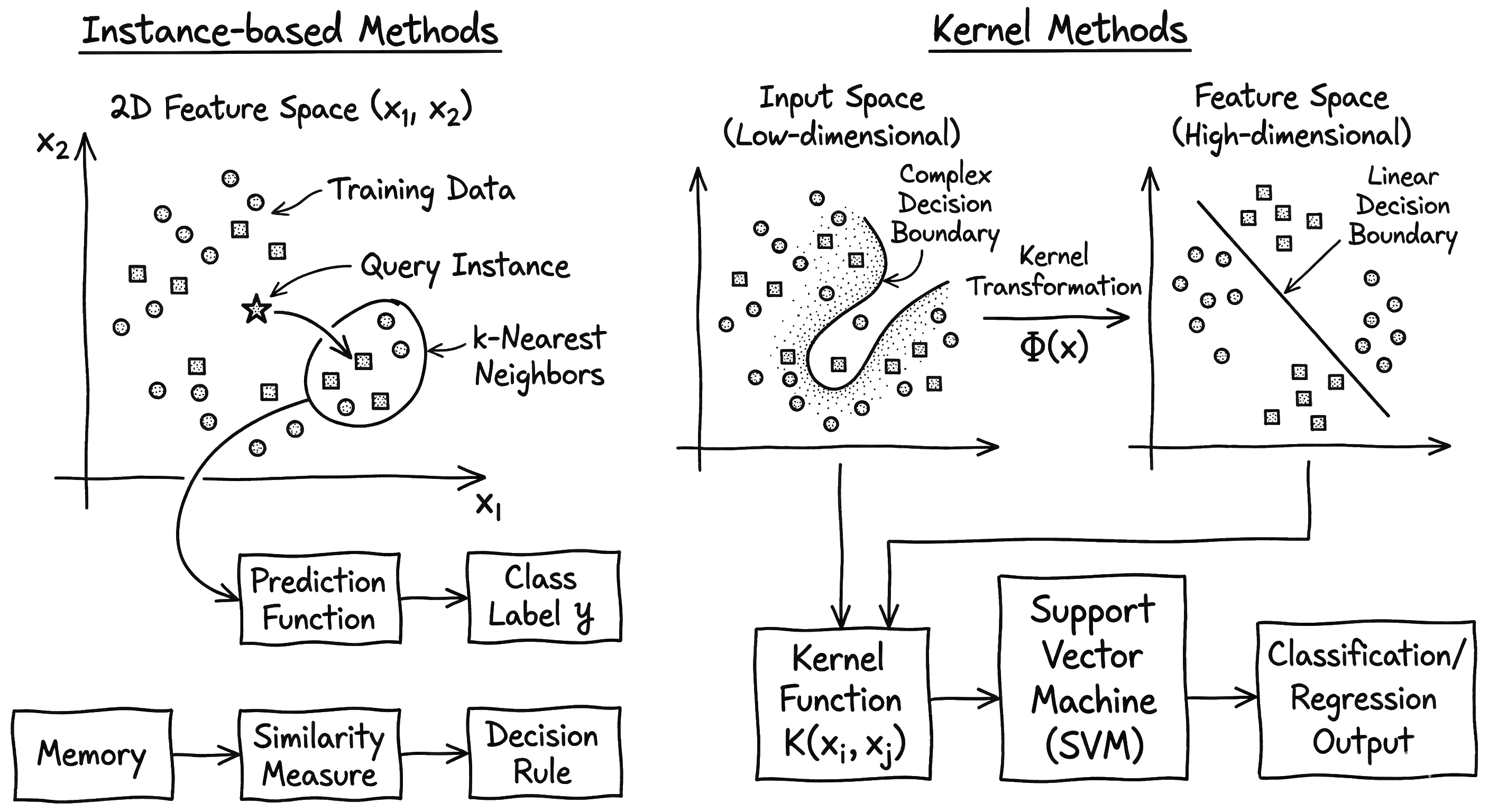
Instance-Based Learning
- Concept:
- “Lazy learning”: No explicit model training phase
- Predictions based on similarity to stored training examples
- Assumptions: Similar inputs yield similar outputs
- Key Components:
- Distance metric (Euclidean, Manhattan)
- Number of neighbors (k)
- Weighting scheme (Uniform vs. Distance-weighted)
k-Nearest Neighbors (k-NN)
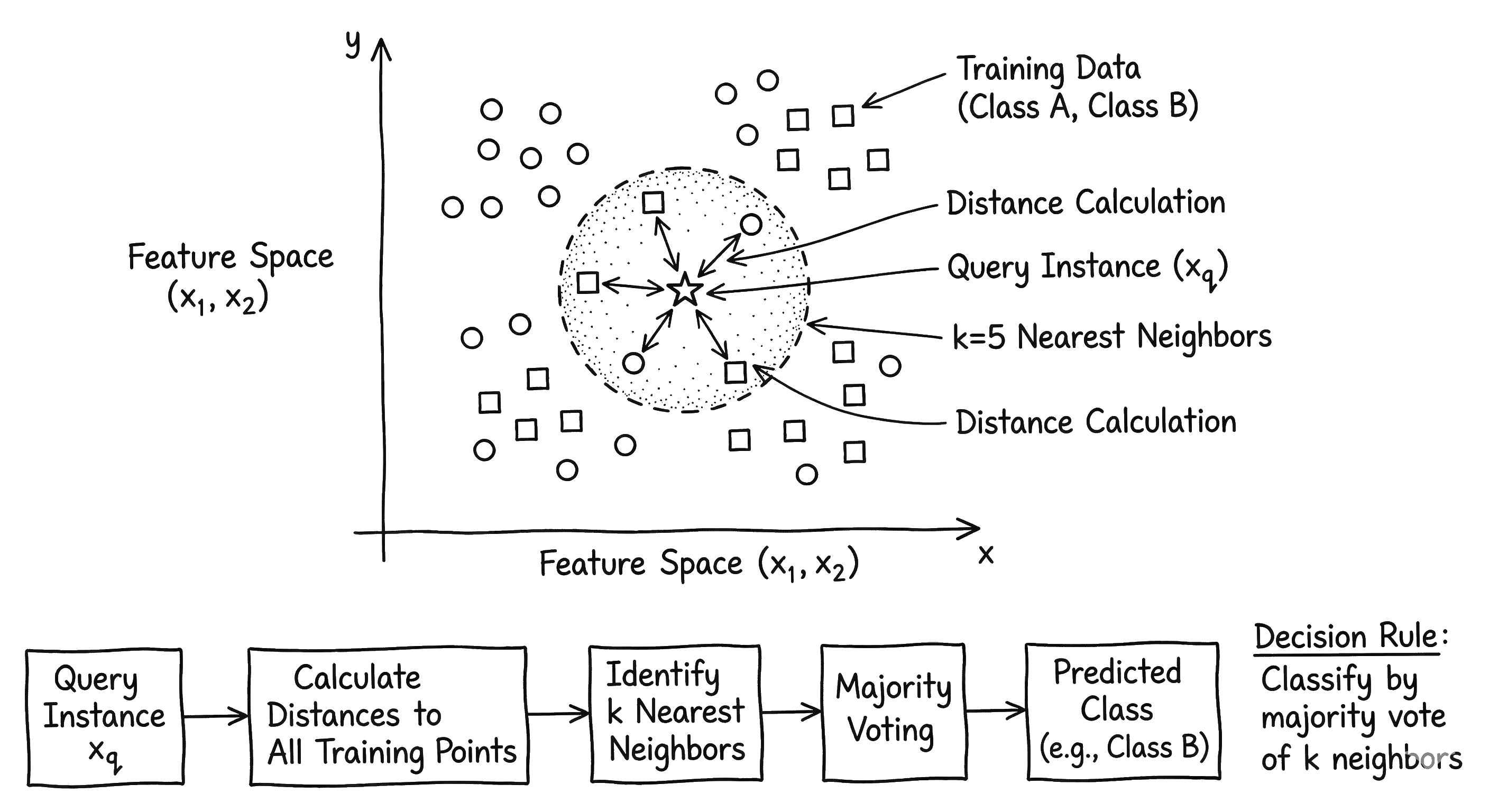
- Algorithm:
- Store all training data
- For a new query point, find the k closest neighbors
- Predict by averaging (regression) or voting (classification)
- Local Similarity Model:
- Adapts to local data density
- Captures complex boundaries without explicit equations
k-NN Considerations
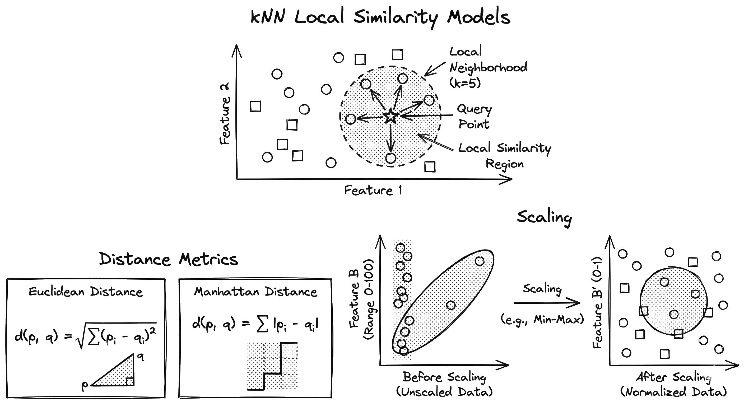
- Distance Metrics:
- Critical choice affecting performance
- Must scale variables appropriately
- Scaling:
- Features with large ranges dominate distance calculations
- Standardization (Z-score) is essential
- Curse of Dimensionality:
- Distance becomes less meaningful in high-dimensional spaces
k-NN Failure Modes
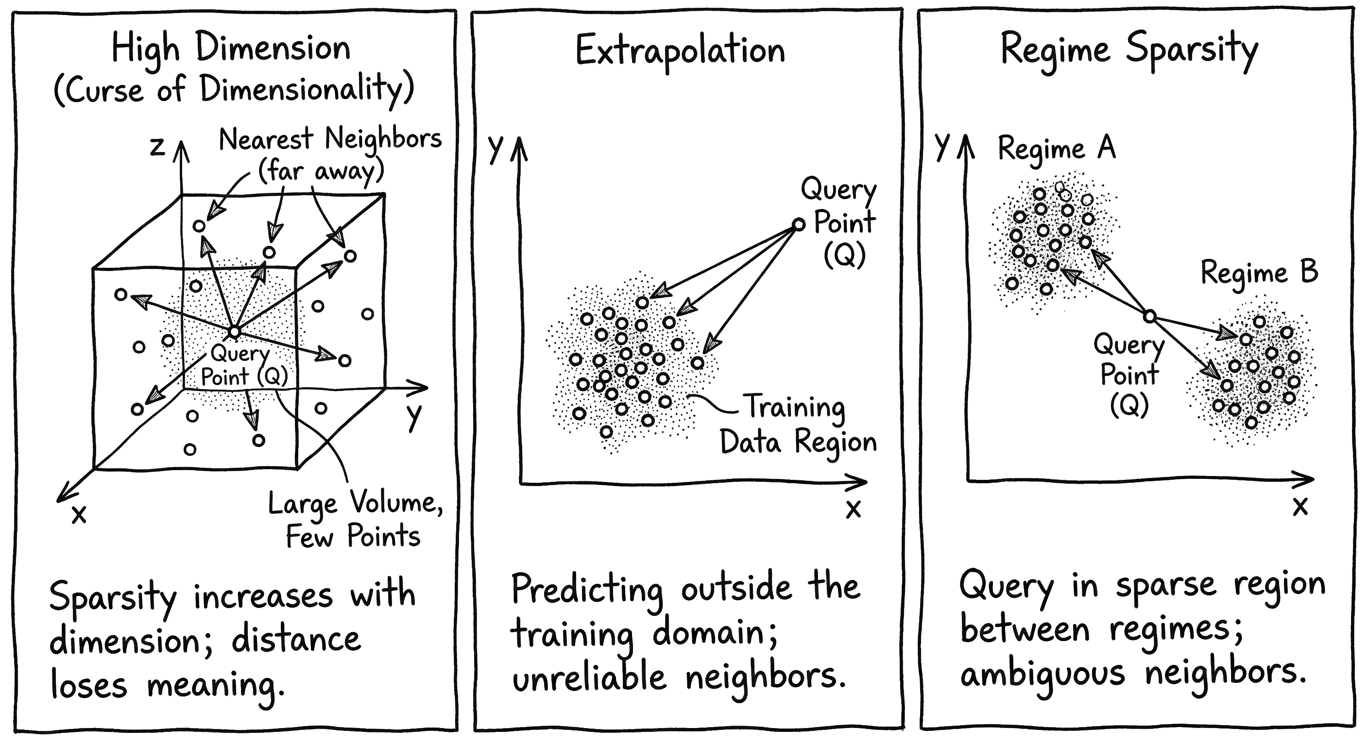
- Issues:
- Sensitive to outliers and noise
- High memory and computation cost at inference time
- Poor performance with sparse data
- Boundary effects at edges of training data
- Requires careful data preprocessing and outlier removal
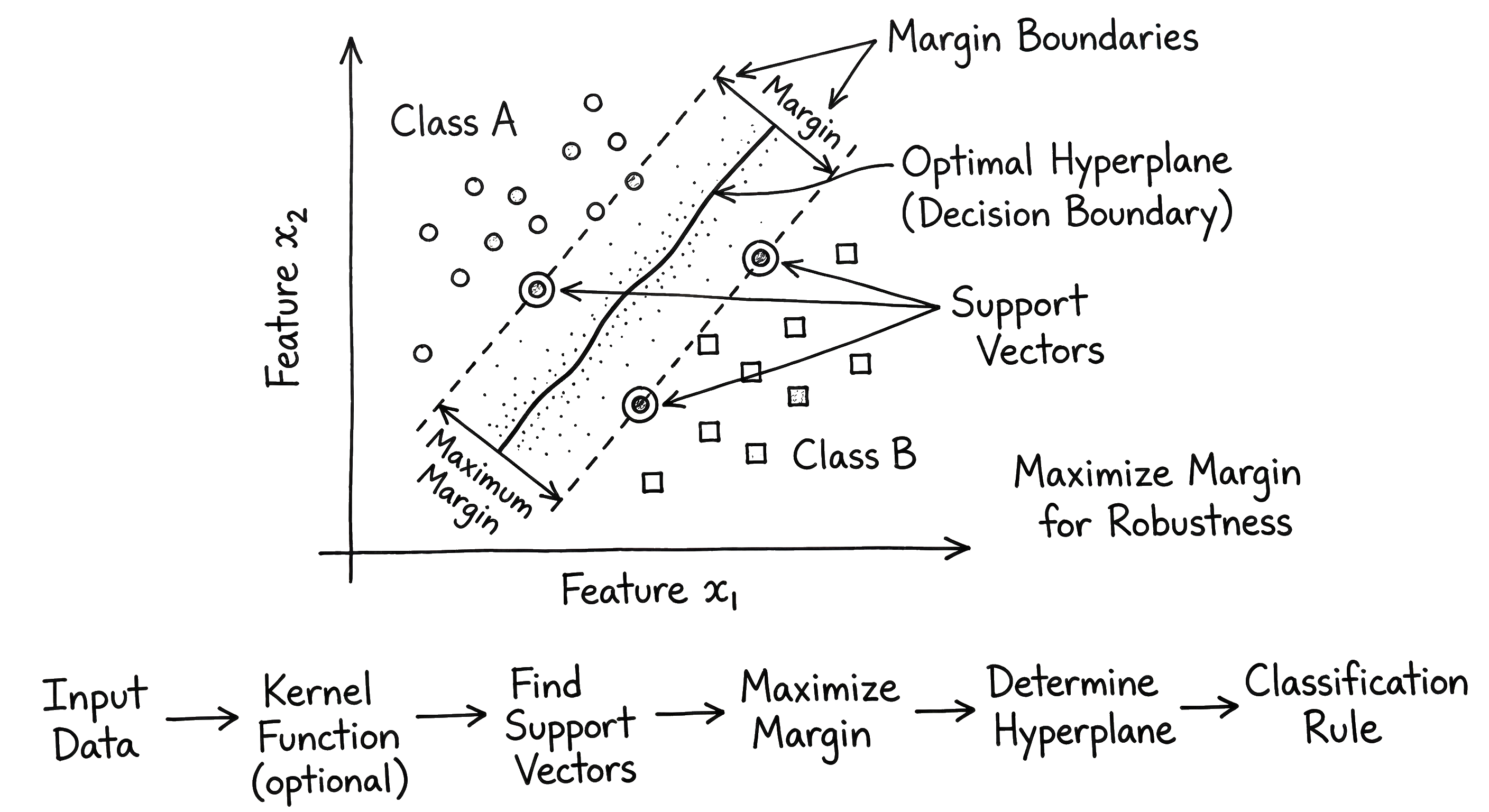
Support Vector Machines (SVM)
- Kernel Method:
- Maps data to high-dimensional space where it is separable
- “Kernel Trick”: Computes dot products without explicit mapping
- Classification:
- Finds optimal hyperplane with maximum margin
- Robust to overfitting due to margin maximization
- Effective for complex, nonlinear boundaries
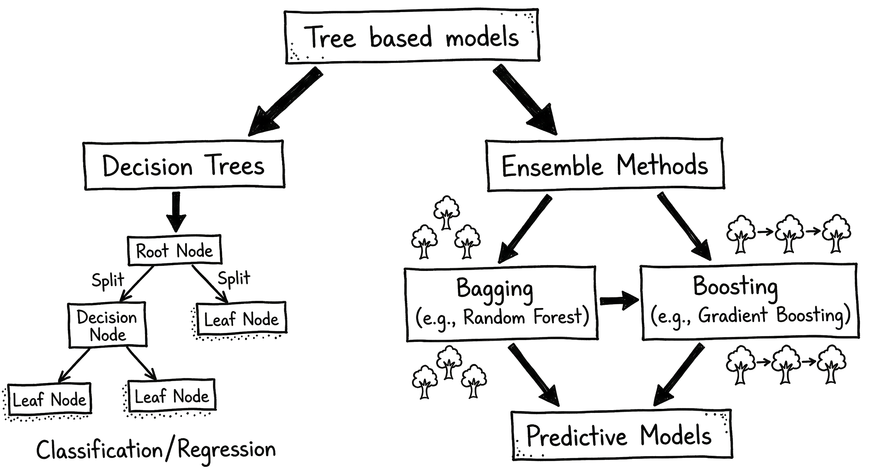
Decision Trees Overview
- Structure:
- Hierarchical set of rules (If-Then-Else)
- Splits data based on feature values
- Leaves represent prediction values
- Advantages:
- Intuitive and interpretable
- Handles mixed data types (numerical/categorical)
- Non-parametric (no distribution assumptions)
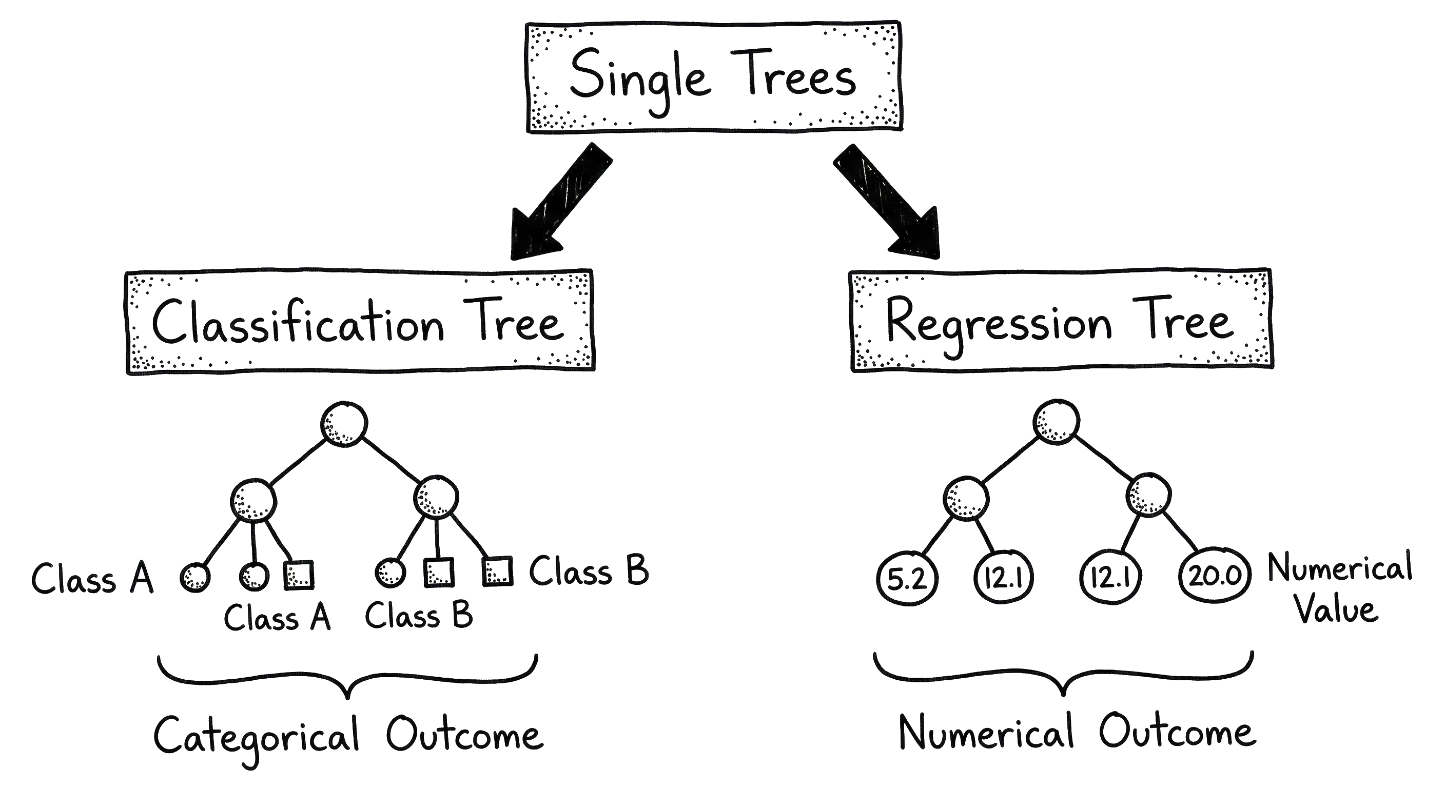
Single Trees
- Construction:
- Recursive partitioning
- Select split that maximizes information gain or minimizes impurity
- Limitation:
- High variance: Small data changes lead to different trees
- Prone to overfitting deep trees
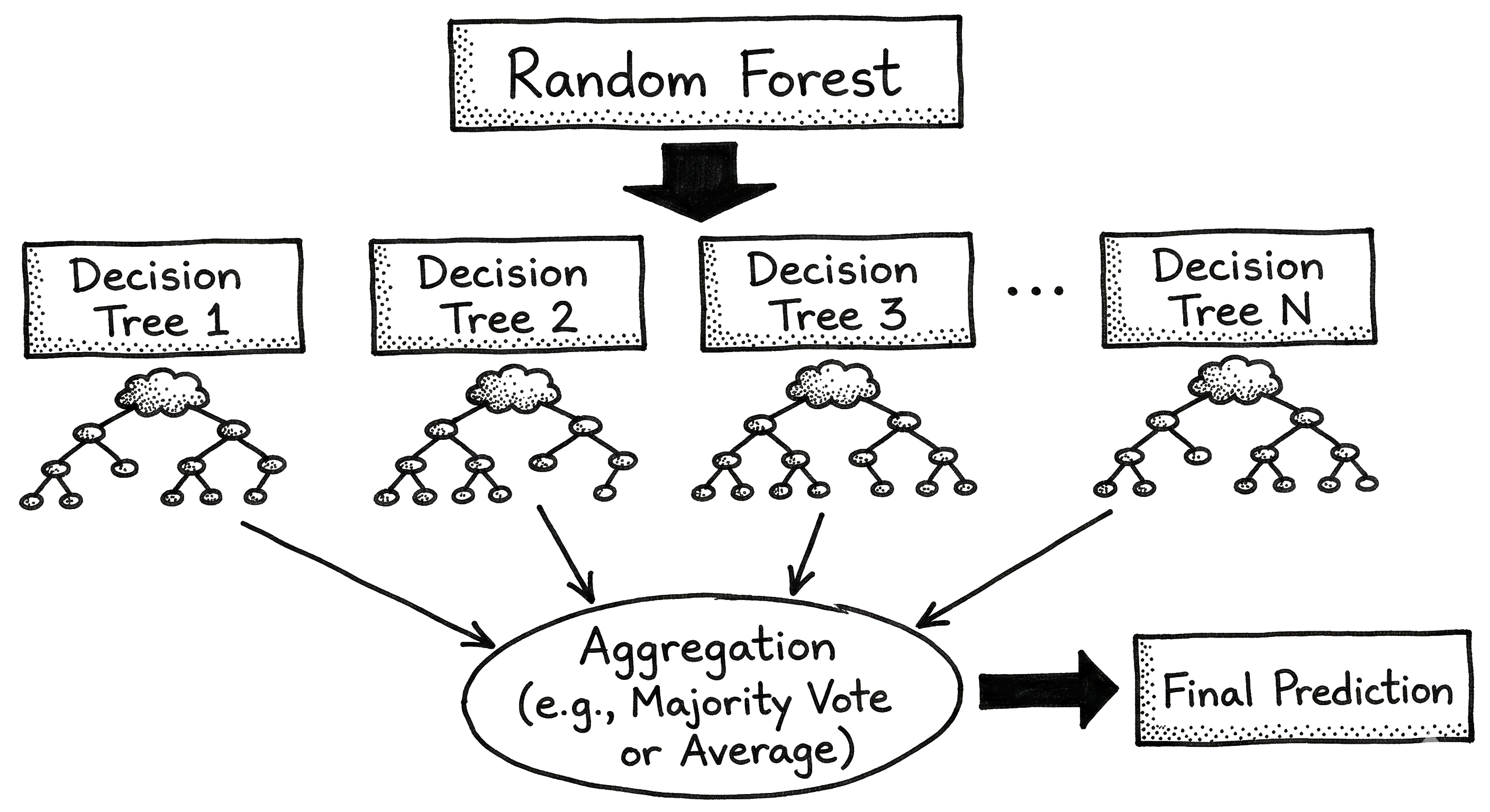
Random Forests
- Ensemble Method:
- Combines multiple decision trees (Bagging)
- Reduces variance and overfitting
- Mechanism:
- Bootstrap sampling: Train each tree on random data subset
- Feature randomization: Split nodes using random feature subset
- Prediction: Average of all tree outputs
Gradient Boosting Trees
- Boosting:
- Sequential training of weak learners (shallow trees)
- Each new tree corrects errors of previous ones
- Variants:
- XGBoost, LightGBM, CatBoost
- Performance:
- State-of-the-art for tabular data
- High accuracy but can overfit if not tuned
.png)
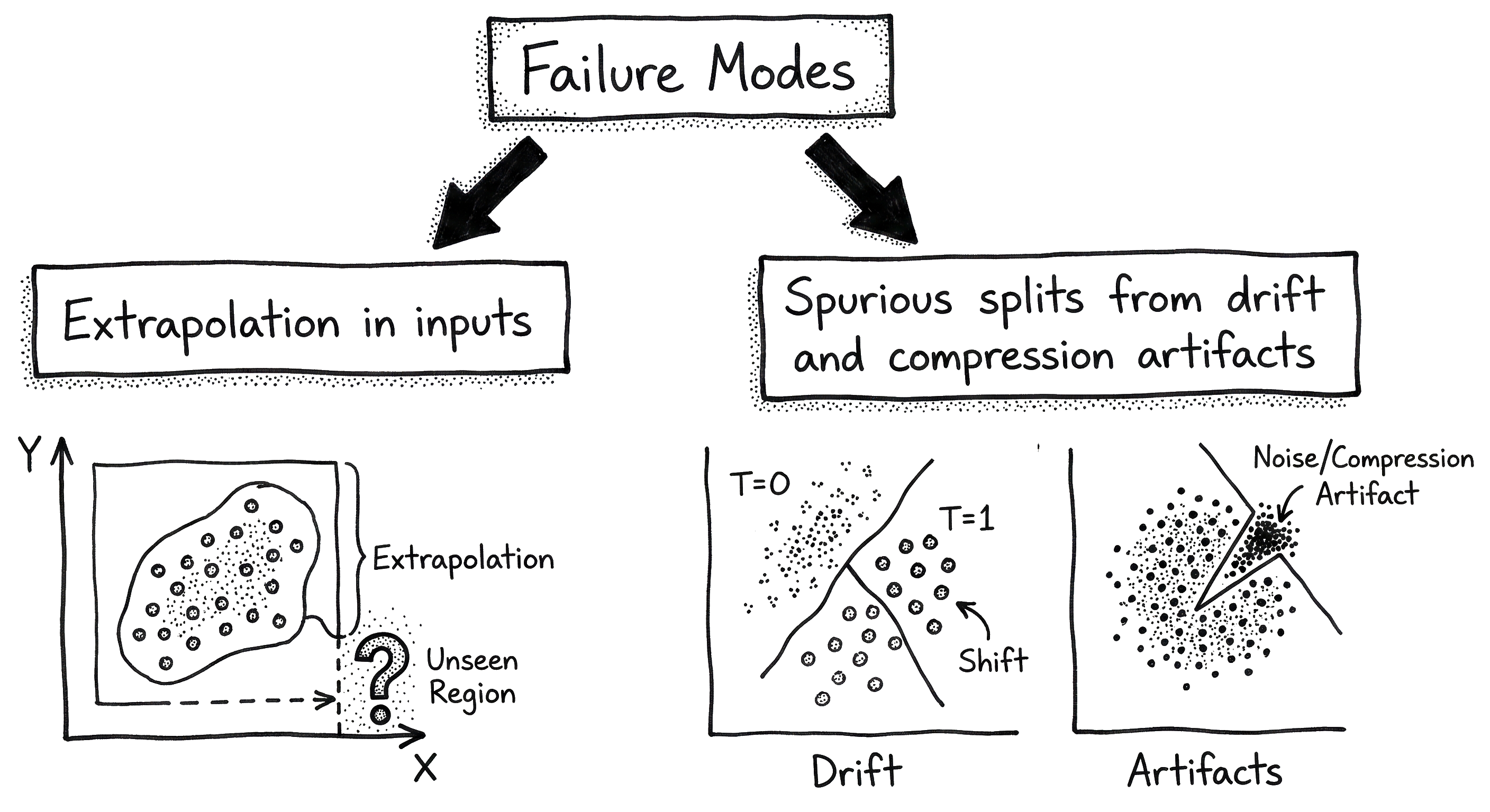
Tree Failure Modes
- Extrapolation:
- Trees cannot predict outside training range
- Constant prediction in unseen regions
- Continuous Functions:
- Approximate smooth functions with step-like outputs
- May need deep trees for smooth transitions
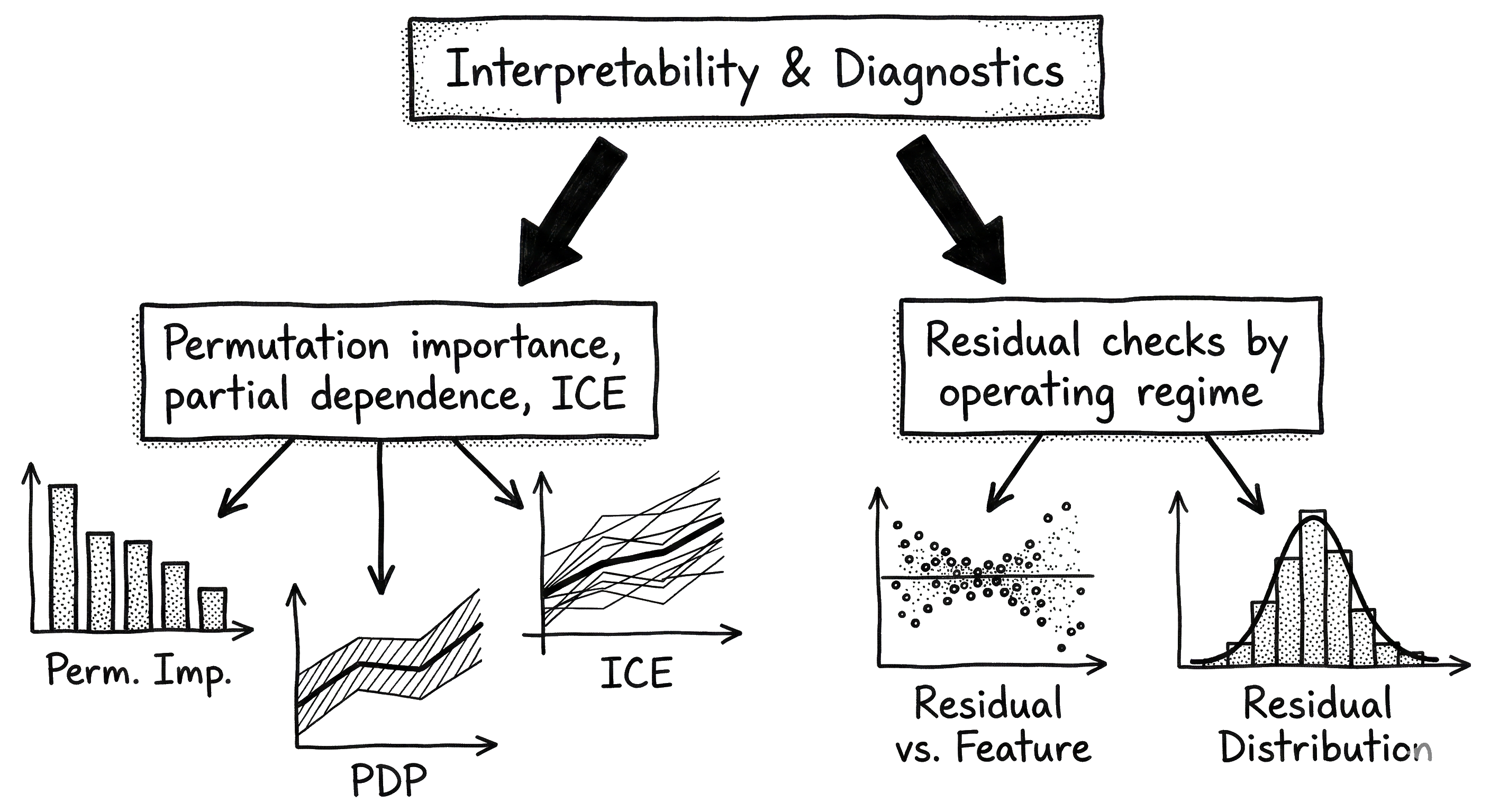
Interpretability and Diagnostics
- Feature Importance:
- Measures contribution of each variable to split quality
- Helps identify key process drivers
- SHAP Values:
- Game-theoretic approach to explain individual predictions
- Shows how each feature pushes prediction from baseline
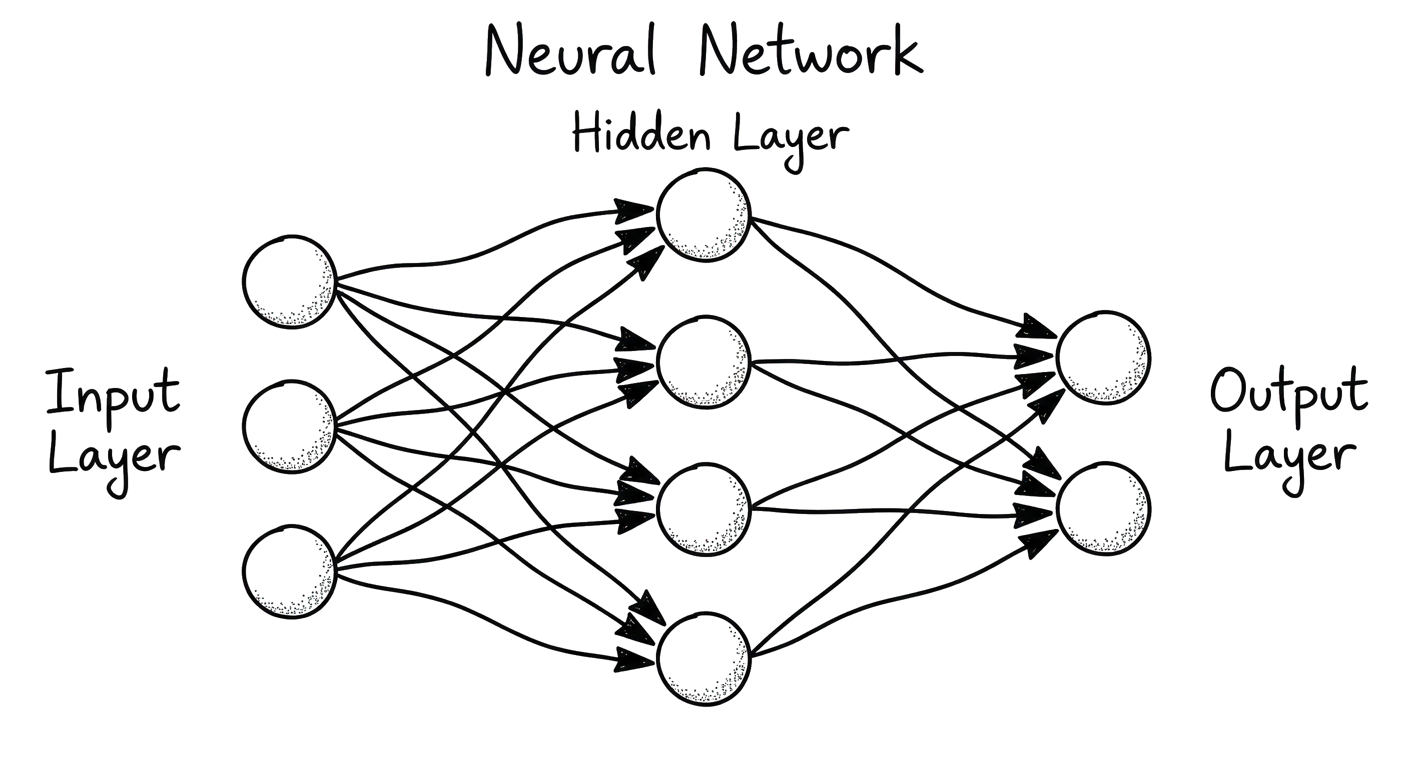
Artificial Neural Networks (ANN)
- Biomimetic Inspiration:
- Mimics biological neurons and synapses
- Universal function approximators
- Structure:
- Layers of interconnected nodes (neurons)
- Weights determine signal strength
- Activation functions introduce nonlinearity (ReLU, Sigmoid, Tanh)
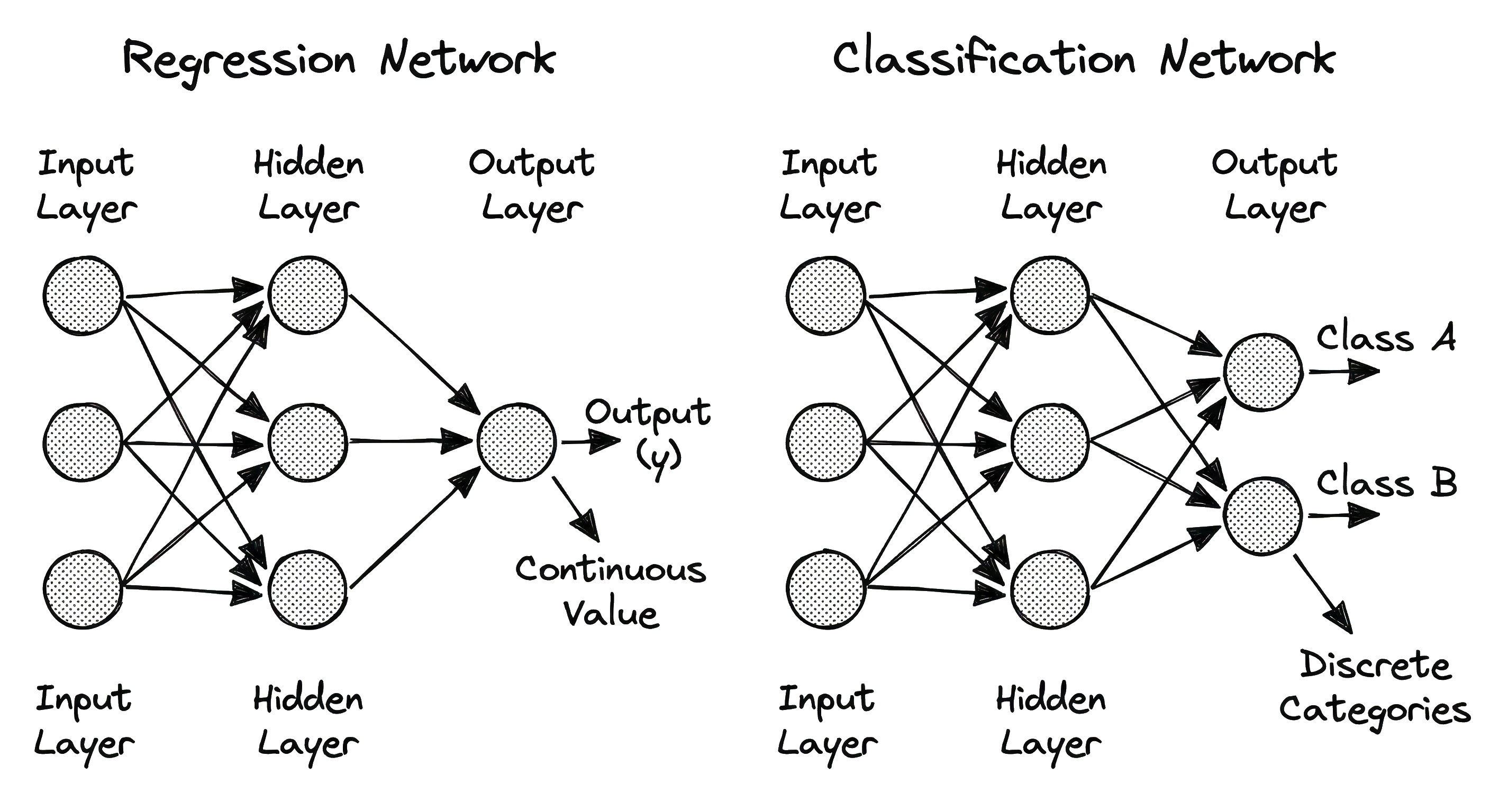
Feedforward Networks
- Architecture:
- Information flows one way: Input \rightarrow Hidden \rightarrow Output
- “Deep Learning” = Multiple hidden layers
- Training:
- Backpropagation algorithm
- Minimize error function (MSE) via gradient descent
- Optimizers: SGD, Adam
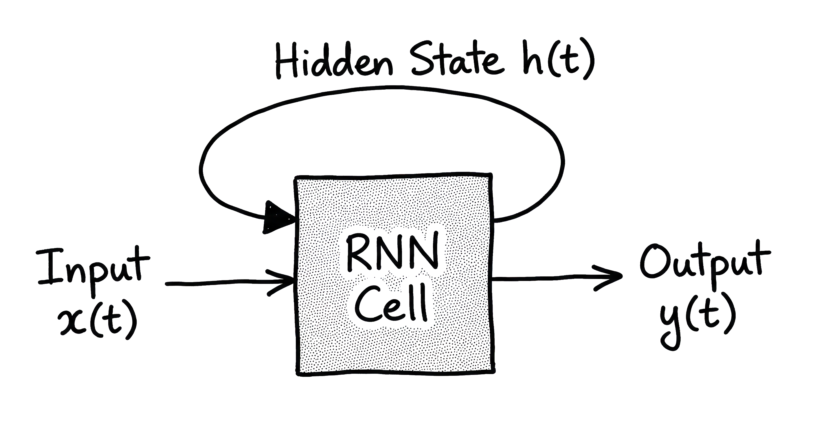
Recurrent Neural Networks (RNN)
- Sequence Processing:
- Designed for time-series and dynamic systems
- Internal memory (hidden state) captures history
- Feedback loops allow information persistence
- Challenge:
- Vanishing gradient problem in long sequences
- Difficult to train on long-term dependencies
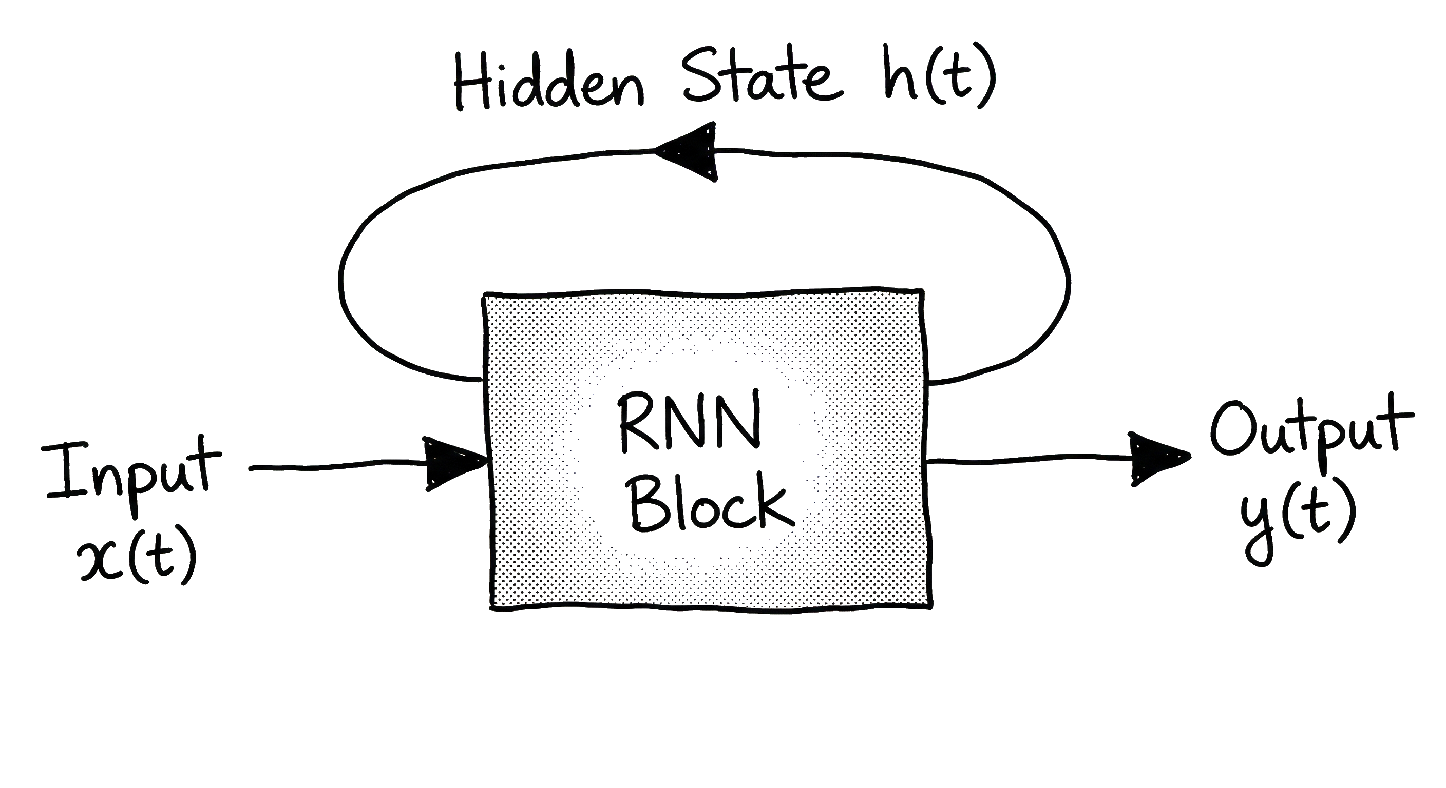
RNN Architecture
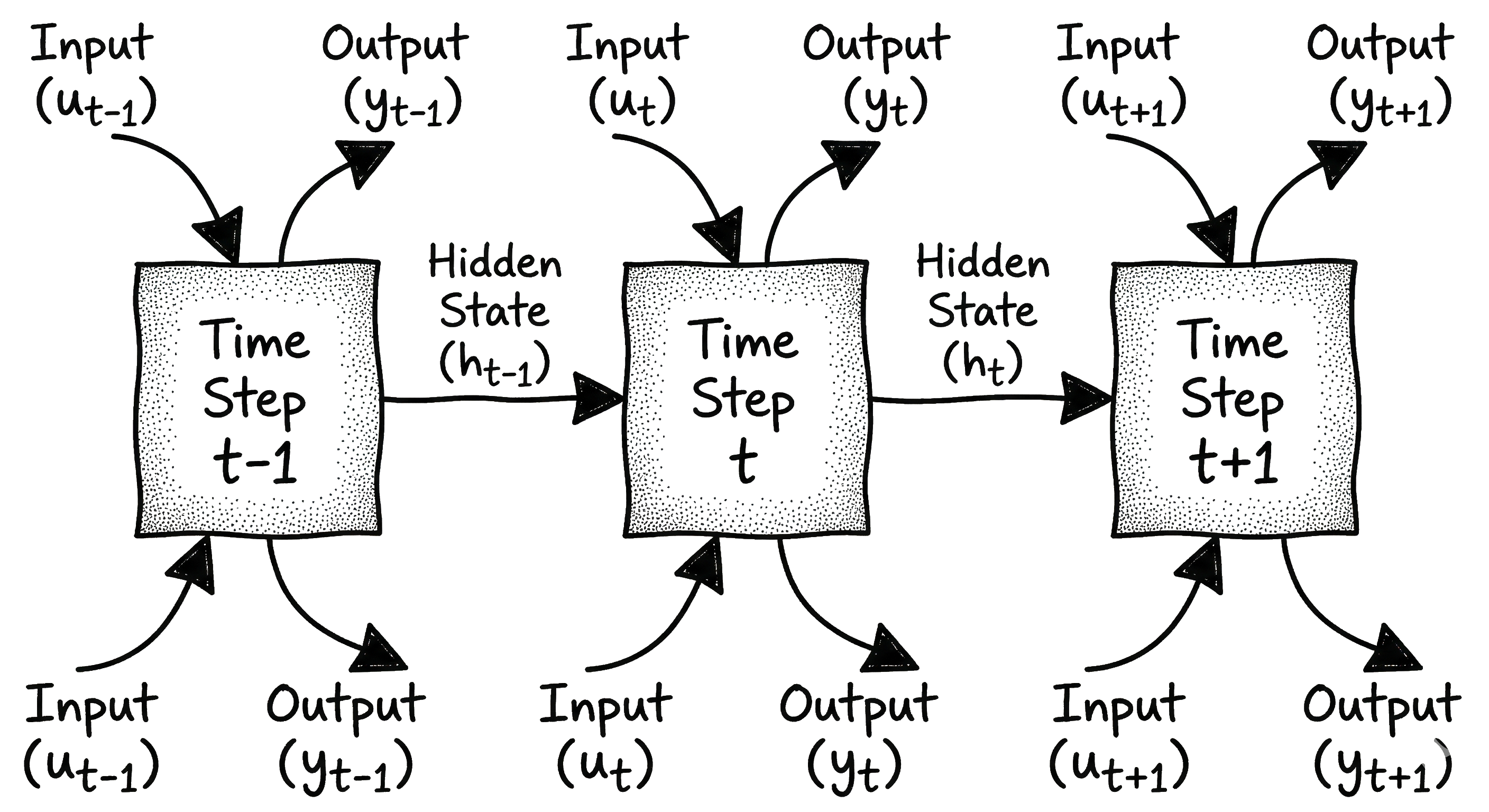
- Unrolled View:
- Can be viewed as multiple copies of the same network
- Each step passes a message to a successor
- Dynamic Modeling:
- Input: Current state x_t + Previous hidden state h_{t-1}
- Output: Prediction y_t + New hidden state h_t
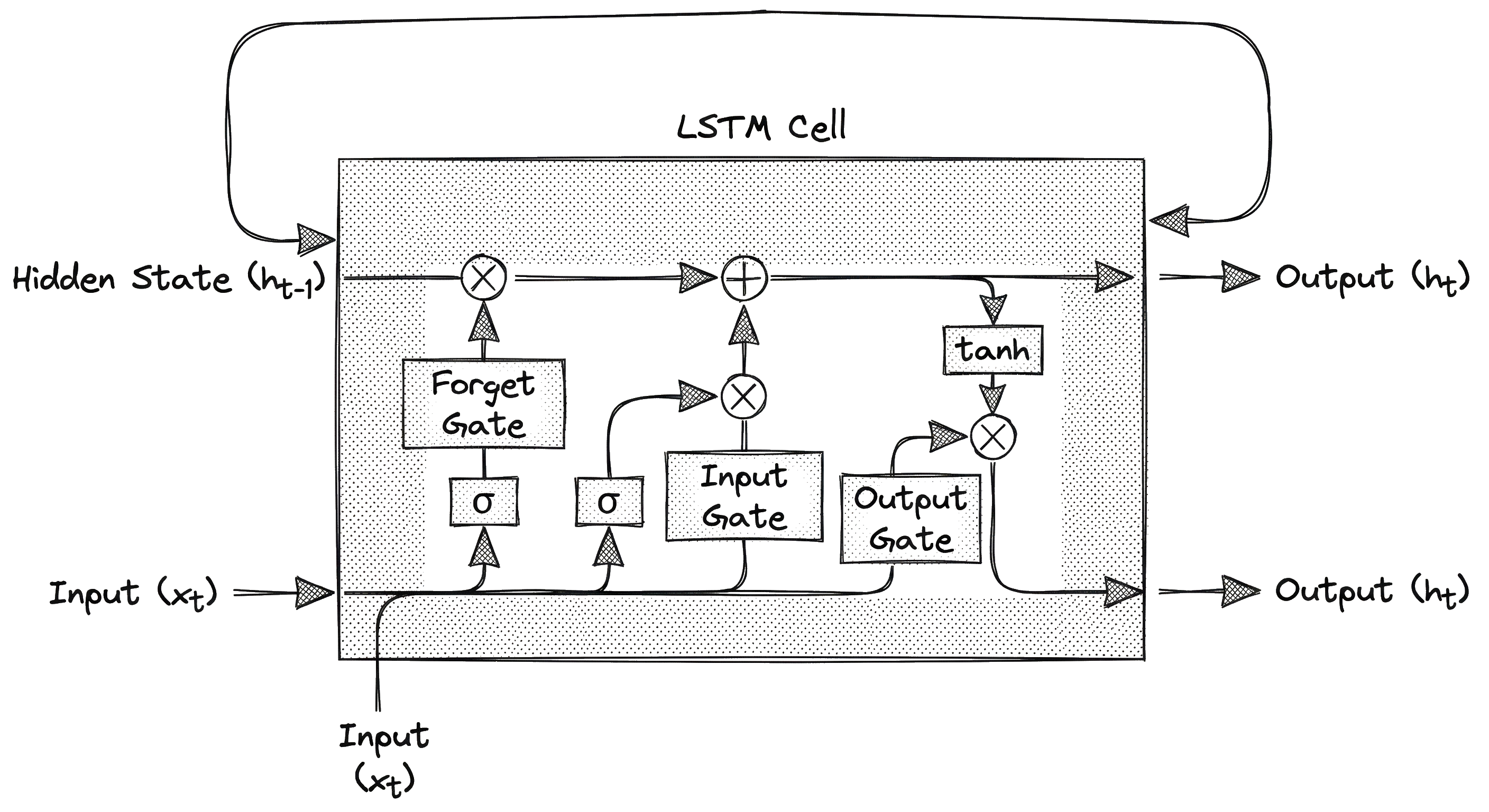
Long Short-Term Memory (LSTM)
- Solution to Vanishing Gradients:
- Specialized gating mechanism controls information flow
- Cell State: Long-term memory highway
- Gates:
- Forget Gate: What to discard
- Input Gate: What to store
- Output Gate: What to output
- Captures lags and long time constants
Gated Recurrent Unit (GRU)
- Simplified LSTM:
- Merges cell state and hidden state
- Combines Forget and Input gates into “Update Gate”
- Benefits:
- Fewer parameters, faster training
- Comparable performance to LSTM for many tasks
- Efficient for industrial time-series data
.png)
Dynamic Modeling Approaches
- NARX Models:
- Nonlinear AutoRegressive with eXogenous inputs
- Uses lagged inputs and lagged outputs as features
- Structure:
- y(t) = f(y(t-1), ..., y(t-n), u(t-1), ..., u(t-m))
- Can use standard FFNN or RNN as the function f
Autoregressive Networks
- Lagged Inputs:
- Explicitly feeding past values creates memory
- Determines model order (how far back to look)
- Design Choice:
- Too few lags: Miss dynamics
- Too many lags: Overfitting, complexity
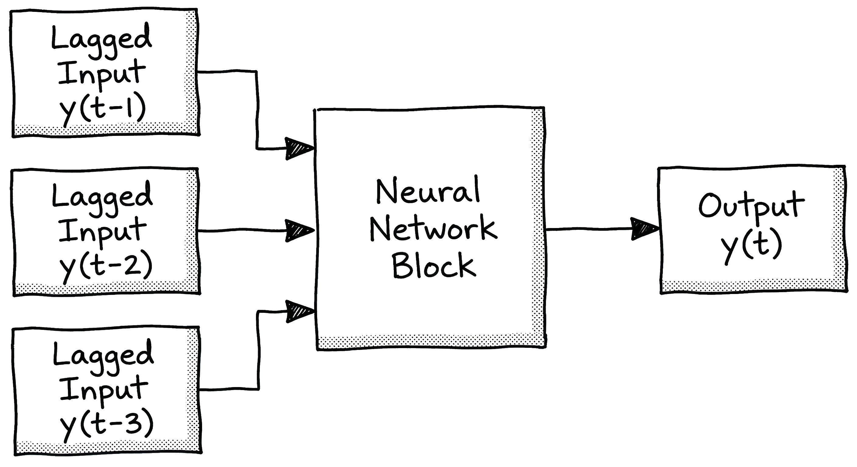
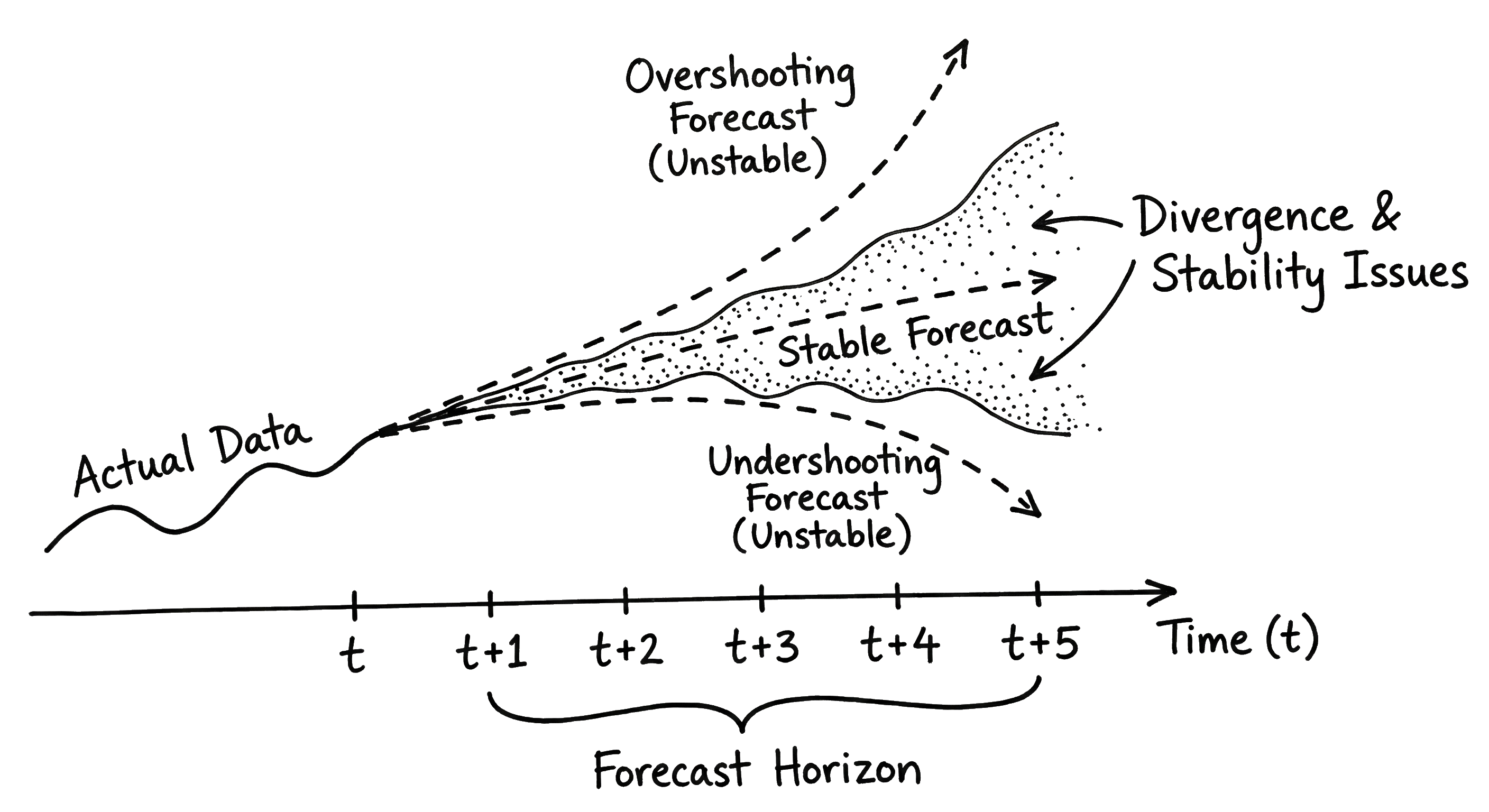
Multi-step Forecasting
- Approaches:
- Recursive: Feed predicted output back as input for next step
- Direct: Separate model for each future step
- Stability Issues:
- Errors accumulate in recursive strategy
- Small biases can lead to divergence over time
- Critical for Model Predictive Control (MPC) usage
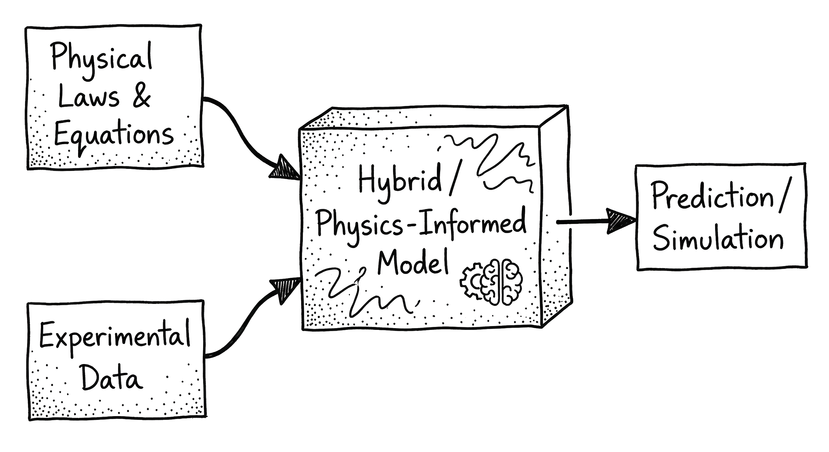
Physics-Informed ML
- Concept:
- Combining First-Principles (White Box) with Data-Driven (Black Box)
- “Grey Box” Modeling
- Motivation:
- Extrapolates better than pure ML
- Requires less training data
- Respects physical laws (mass/energy conservation)
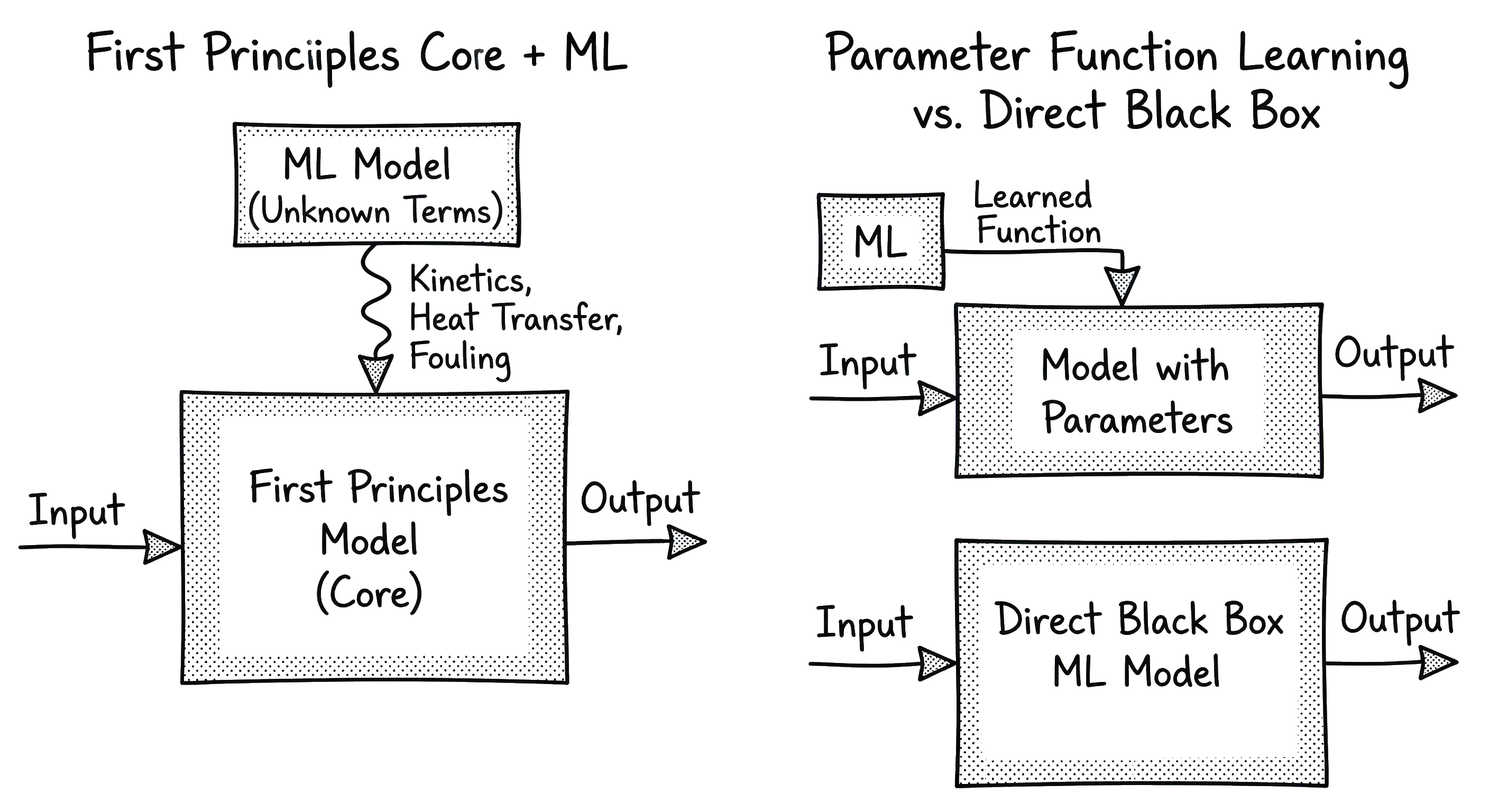
Serial Hybrid Structure
- Architecture:
- ML estimates unmeasured parameters/states
- Physics model uses these inputs for final prediction
- Example:
- NN predicts reaction rate from temperature/concentration
- ODE solver integrates mass balance using NN rate
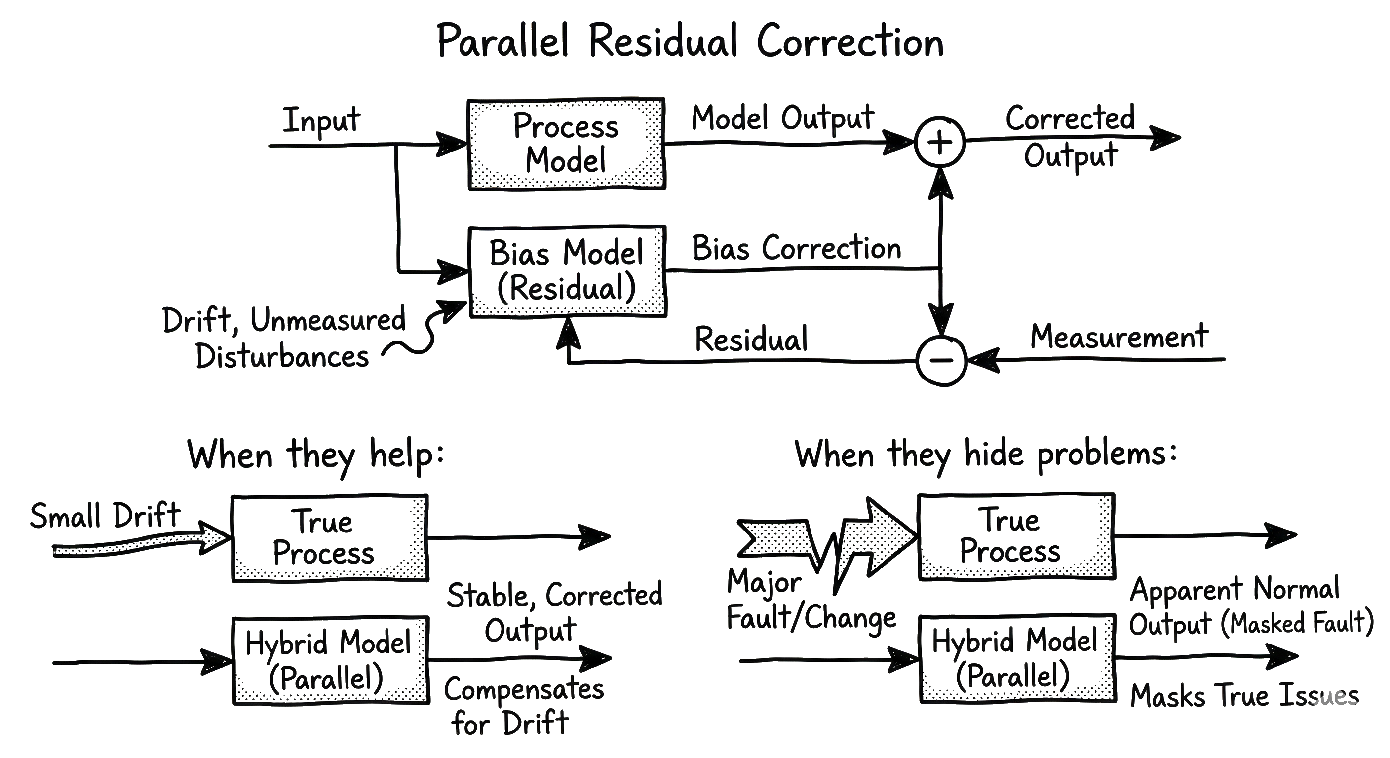
Parallel Residual Correction
- Architecture:
- Physics model gives baseline prediction
- ML model predicts the residual (error)
- Final Output = Physics + ML Correction
- Use Case:
- Correcting simplified physics assumptions
- Capturing unknown disturbances
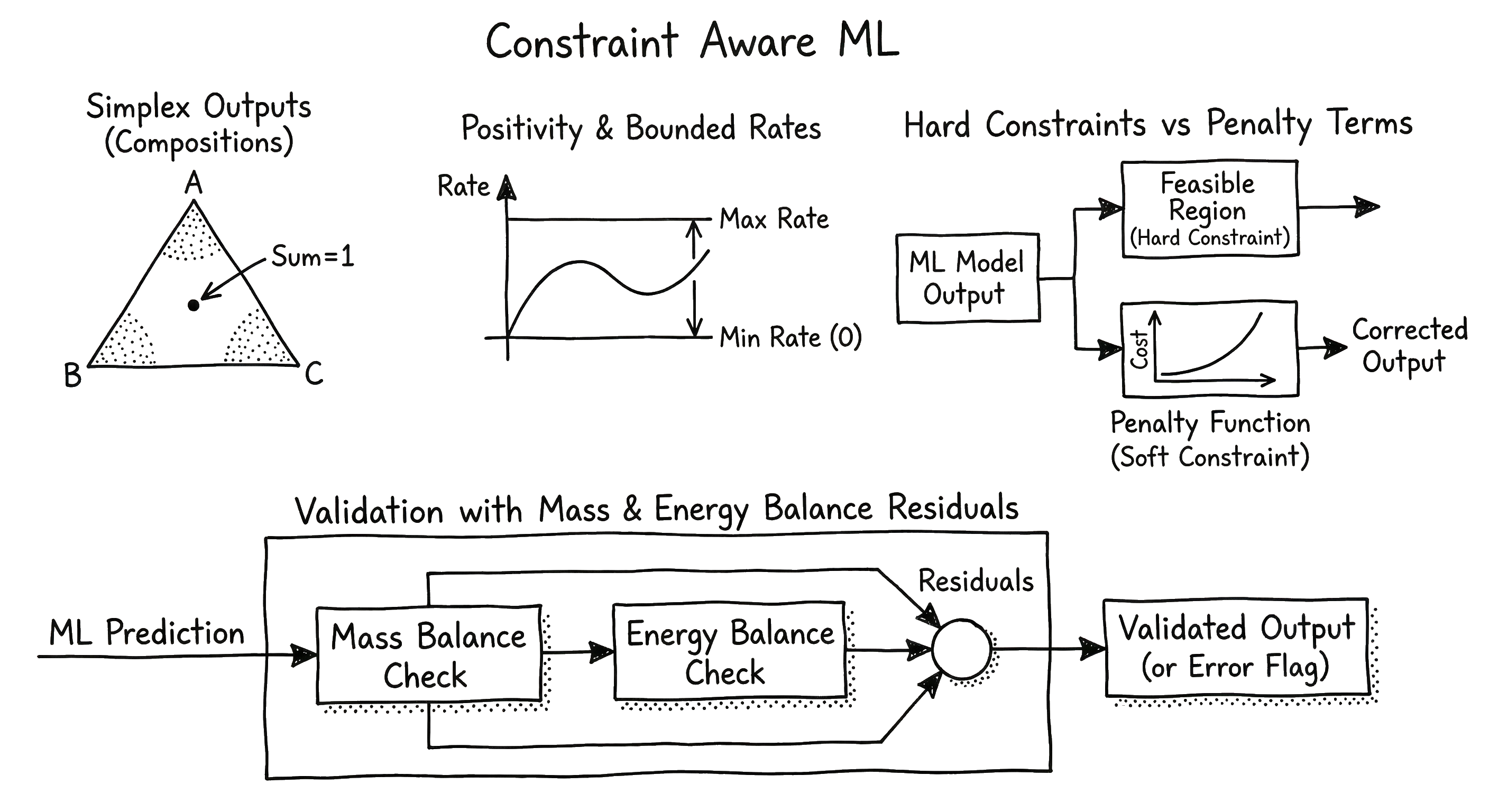
Constraint-Aware ML
- Problem: Pure ML output can violate physical limits (e.g., negative concentration)
- Solutions:
- Hard Constraints: Output layers with bounds (e.g., ReLU for positivity)
- Soft Constraints: Loss function penalties for physics violations
- Ensures physical consistency of predictions
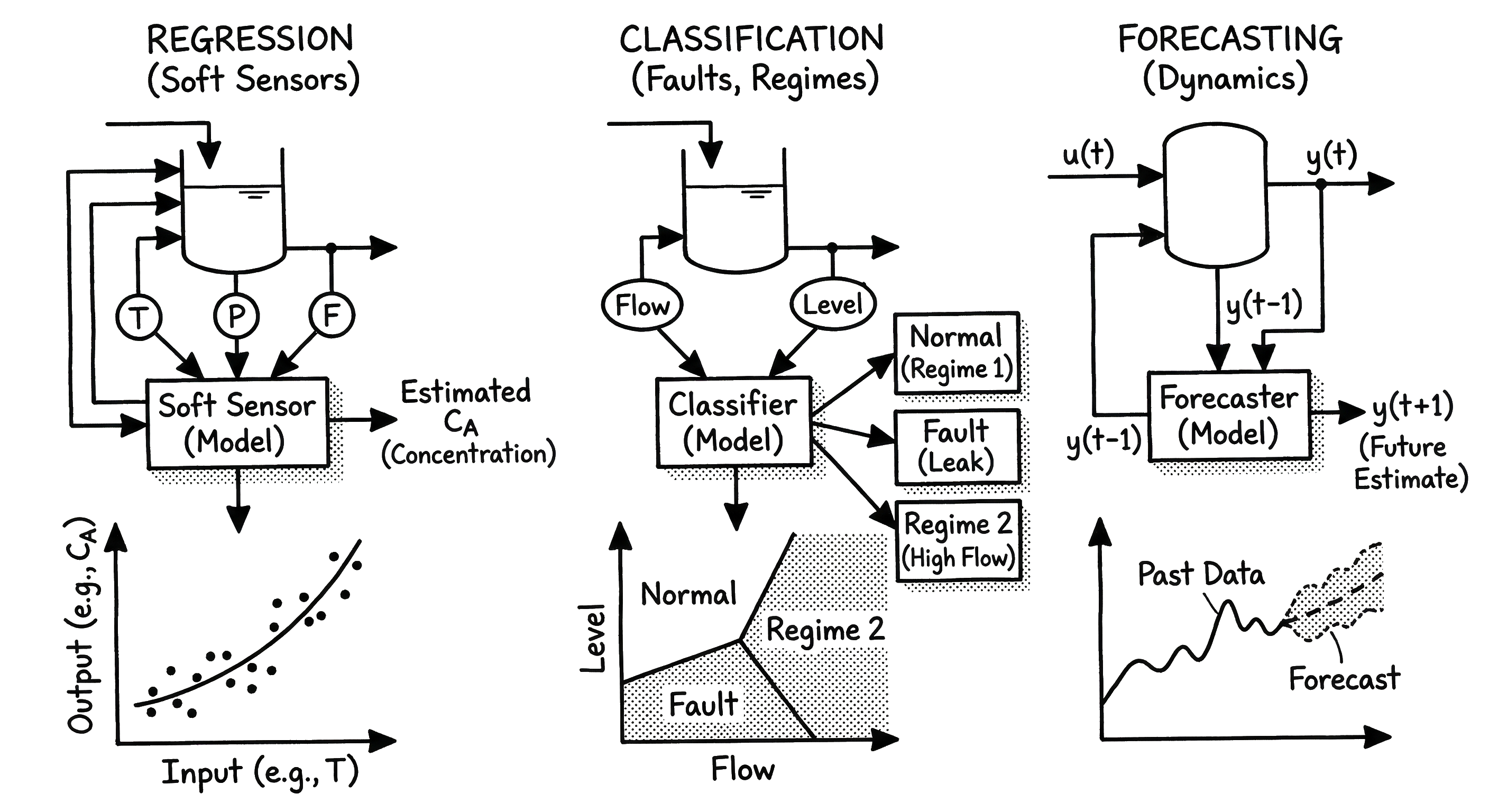
Model Selection & Validation
- Data Splitting:
- Training: Fit parameters
- Validation: Hyperparameter tuning
- Testing: Final performance check
- Metrics:
- RMSE, MAE, R^2
- Visual inspection of residuals
- Cross-Validation:
- K-Fold or Time-Series Split
- robust error estimation