3 Introduction
3.1 Nature of chemical processes
Chemical processes greatly influence every aspect of our life. All important industrial sector such as food production, water treatment, healthcare and pharmaceuticals, energy, automotive industry, and so on rely on chemical process industry to supply ingredients, raw materials, and enabling technologies. In recent years, significant attention is given to sustainability in the chemical process industry. New processes and retrofit of existing processes are based on responsible resource utilization, minimization of environmental impact, and considerations to long-term viability and competitiveness. Chemical processes involve several unit operations, such as mixing, heat exchange, mass transfer, and reaction. In a chemical process, required unit operations are performed in a specific sequence to achieve specific objectives.
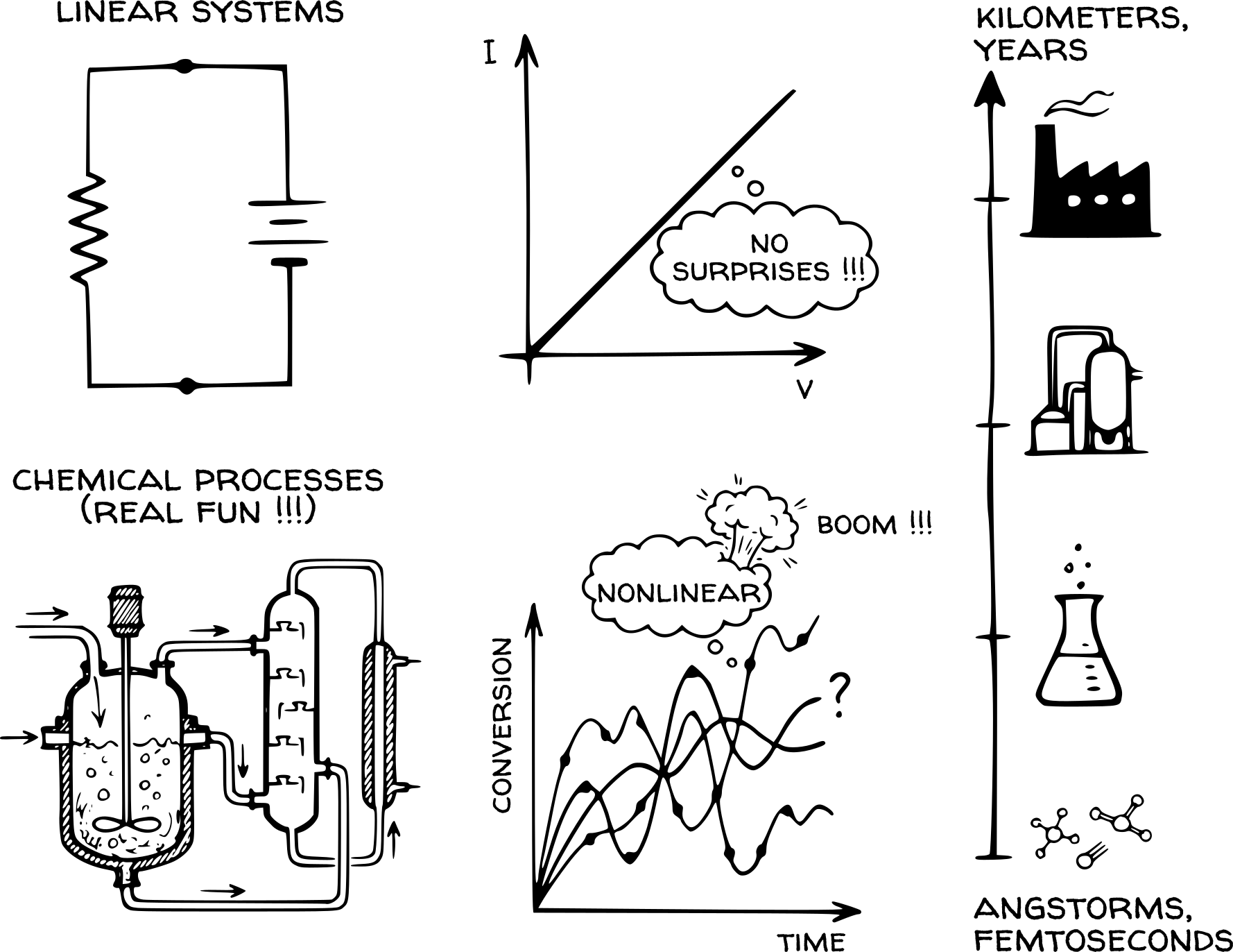
Many engineering systems such as mechanical assemblies, electrical circuits, and control systems are deterministic and linear, which means that the output is directly proportional to the input. For example, electrical resistors follow Ohm’s law (\(V=IR\)) and ideal springs obey Hooke’s law (\(F=kx\)). This linearity makes the system’s behavior easy to predict. If an input is doubled, the response doubles; if two inputs are applied at once, their effects simply add up. This mathematical convenience allows engineers in these fields to design complex systems by combining simple, well-understood components with high confidence.
Unlike linear systems, a chemical process involves the transformation of matter and energy at the molecular level, governed by probabilistic molecular events (stochastic thermodynamics and kinetics). This stochastic nature contributes to the inherent complexity of chemical processes. Additionally, chemical processes exhibit strong non-linearity arising from multiple sources. For example, reaction rates follow exponential temperature dependencies (e.g., Arrhenius kinetics), phase equilibria involve non-linear thermodynamic relationships, and transport phenomena like heat and mass transfer are governed by non-linear driving forces. When the processes operate in relatively narrow ranges, their behavior may appear approximately linear, but the non-linearity often becomes apparent during process upsets and disturbances. Therefore, simple linear deterministic models are usually insufficient for representing chemical processes. Moreover, chemical processes are often multivariable and tightly coupled. This means that changing one variable can affect multiple outputs, and isolating variables for analysis is often difficult. Consider a distillation column. Increasing the reflux rate improves product purity but simultaneously decreases top temperature, increases reboiler duty, and alters the internal vapor-liquid hydraulic balance. A single change in parameter propagates through energy, pressure, and composition profiles, making variable isolation impossible. This also has a knock-on effect on downstream unit operations in the process.
Chemical processes are inherently dynamic, meaning their behavior changes over time. Apart from process dynamics, operating conditions and equipment health also change over time. For example, in the Haber-Bosch ammonia synthesis, the iron catalyst undergoes thermal sintering and structural rearrangement over its lifespan (~ 4 to 5 years), necessitating a gradual increase in reactor temperature to compensate for lost activity. A model tuned for fresh catalyst may not be suitable for older catalyst. Heat exchanger surfaces foul over months, increasing thermal resistance. This reduction in heat transfer efficiency forces the control system to increase utility flow rates to maintain target outlet temperatures. Consequently, the overall heat transfer coefficient (\(U\)) acts as a time-varying parameter rather than a constant. A static model that assumes a clean exchanger will progressively drift from reality, failing to predict the true energy demand. Ambient temperatures swing daily. A model trained on summer data may fail spectacularly in winter.
This complexity is further intensified by the vast range of time and length scales involved. As illustrated in Figure 3.1, phenomena occur simultaneously from the molecular level (angstroms, femtoseconds) to the unit operation level (meters, hours) and up to the plant lifecycle (kilometers, years). Effective models must bridge these disparate scales to accurately capture how microscopic events drive macroscopic performance.
3.2 Modeling of chemical processes
It is clear from the preceding discussion that chemical processes are inherently complex. They exhibit non-linear relationships between variables, tight coupling where one change affects multiple outputs, dynamic behavior that evolves over time, and phenomena occurring across multiple scales. These characteristics make chemical processes challenging to design, difficult to predict, hard to control, and complex to optimize.
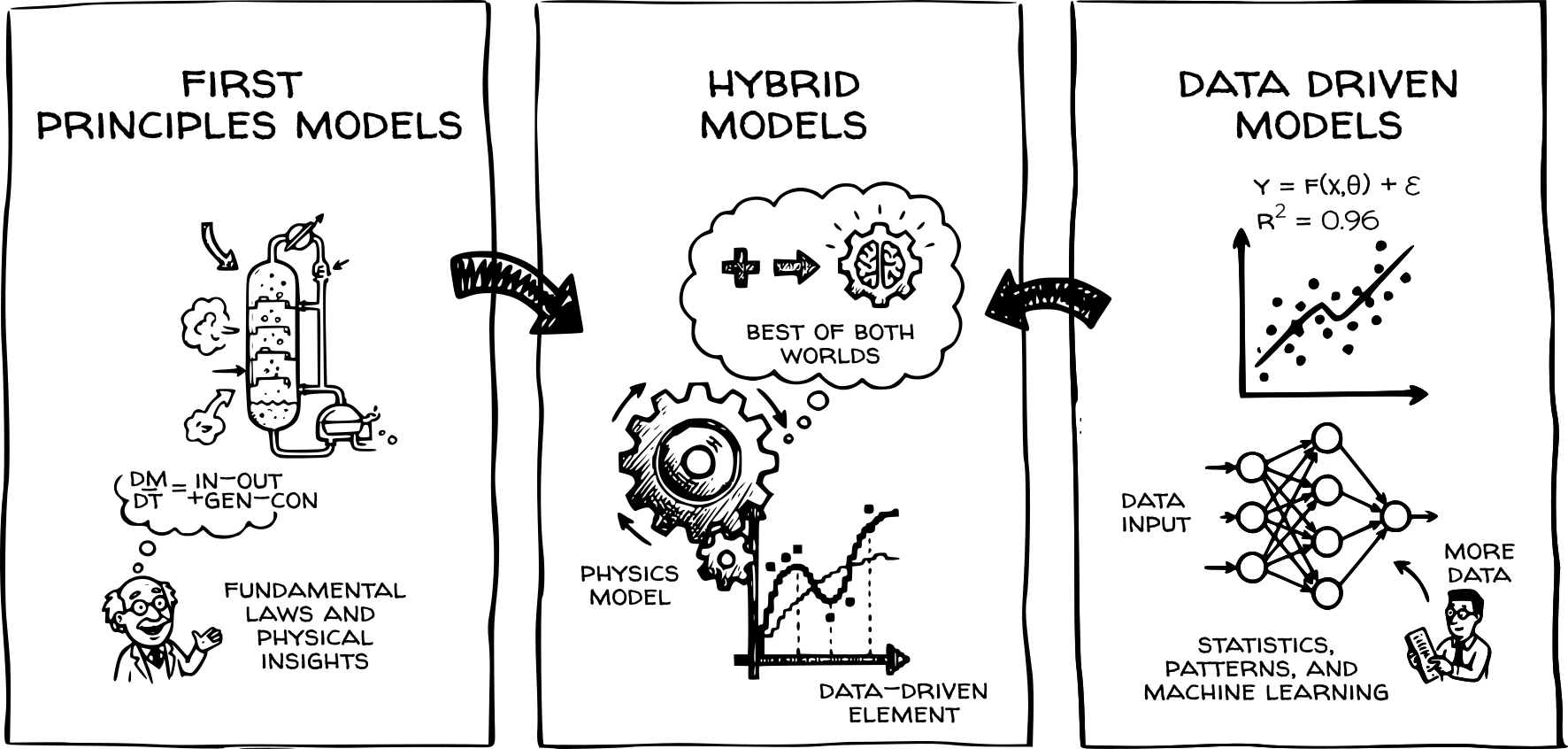
Computational/ Process models address these challenges. Models enable engineers to simulate process behavior, predict responses to disturbances, design effective control strategies, and optimize operations for safety, product quality, and efficiency. These models can be broadly classified as mechanistic or first-principles models (based on fundamental physical and chemical laws, spanning from molecular simulations to computational fluid dynamics to process-level mass and energy balances), empirical or data-driven models (derived from experimental or operational data using statistical or machine learning techniques), or hybrid approaches that combine both paradigms, as depicted in Figure 3.2.
3.2.1 First-principles models
Historically, chemical engineers have relied heavily on first-principles models. These models are derived from the conservation laws of mass, energy, and momentum. First principles models are also known as mechanistic models, phenomenological models or as white-box models in system engineering. These models have been discussed at length in excellent textbooks such as Luyben (1990), Aris (1999), Hangos and Cameron (2001), and Upreti (2017). Therefore, we will not discuss them in detail here.
First-principles models formalize conservation laws of mass, energy, and momentum into mathematical equations. Conservation laws are accompanied by constitutive equations that define transport rates (e.g., Fourier’s law for heat, Fick’s law for mass), reaction kinetics (e.g., Arrhenius expressions), and thermodynamic equilibria (e.g., equations of state, phase equilibrium). These mathematical formulations produce systems of algebraic equations (e.g. steady state balances), ordinary differential equations (ODEs) (e.g. lumped dynamic behavior), and partial differential equations (PDEs) (e.g. distribution in space and time). The equations can appear individually or in combination, depending on the spatial and temporal complexity of the process. Inequality constraints enforce physical limits such as monotonicity, convexity, non-negativity of state variables. The systems of equations essentially encode how process variables evolve in response to controlled inputs and external disturbances.
Generally, every parameter in the first-principles model has a physical meaning. For example, heat transfer coefficient, reaction rate constant, etc. Therefore, one can interpret the model parameters and understand the process behavior. Moreover, since these models are grounded in fundamental physical laws, they usually hold true even outside the range of conditions for which they were developed and validated for.
However, they are not without their limitations. For example, they are often difficult to develop and require significant domain expertise. This is especially true for complex processes with limited understanding of the underlying mechanisms. Coupling phenomena across different scales, such as molecular, equipment, and plant levels, introduces high-dimensional systems. Spatial and temporal discretization of these equations, along with discrete events, dead times, parameter uncertainties, and stiff dynamics makes them computationally expensive to solve. Even when fundamental equations are known, the resulting plant-model mismatch and computational expense often prevent deployment in online control and optimization.
Despite of these challenges, first-principles models have successfully guided the design and operation of complex chemical processes for over 75 years and still remain essential indispensable when data is scarce or expensive. Process development, scale-up, and optimization of novel processes require predictions beyond historical operating ranges, pure data-driven models perform poorly in these scenarios. First principles models also enable analysis of rare events (runaway reactions, equipment failures) that cannot be safely observed. Even in data-rich environments, these models provide physical bounds that constrain data-driven predictions and improve their reliability.
3.2.2 Data-driven models
Data-driven models adopt a fundamentally different approach to process representation. Rather than deriving equations from physical laws, these models identify statistical relationships between measured process variables. The rise of distributed control systems, industrial sensors, and data historians has made large volumes of operational data available at minimal cost. Machine learning and statistical regression techniques exploit this data to construct input-output mappings without requiring explicit mechanistic knowledge. These models are particularly effective when physical phenomena are too complex to model from first principles, when process mechanisms are poorly understood, or when rapid model development is required.
Traditional empirical modeling in chemical engineering relies on statistical regression techniques. Linear regression and partial least squares (PLS) capture linear relationships between process variables, with PLS specifically designed to handle high-dimensional predictor spaces common in process data. Polynomial regression extends linear frameworks through basis expansion to approximate smooth nonlinearities (Montgomery, Peck, and Vining 2013). Time-series models such as auto regression moving average with exogenous variables (ARMAX), state-space representations (Box, Jenkins, and Reinsel 2008) incorporate autoregressive structures and moving-average components to capture temporal dynamics, feedback loops, and serial correlation inherent in chemical processes. These methods offer computational efficiency, theoretical guarantees on parameter estimates (confidence intervals, hypothesis testing), and interpretability through explicit coefficient analysis.
Unlike classical regression methods that require pre-specifying functional forms (linear, polynomial, exponential), modern machine learning methods learn relationships directly from data. Neural networks build layered representations that can approximate arbitrary relationships between process variables. Tree-based ensemble methods (random forests, gradient boosting) automatically identify decision boundaries and operating regime transitions without requiring manual feature selection. Support vector machines handle classification and nonlinear regression through kernel-based transformations. These methods capture complex process behavior and variable interactions more flexibly than classical regression but provide limited insight into underlying mechanisms and behave unpredictably outside training conditions.
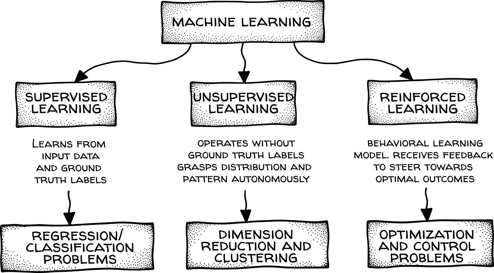
Data-driven models can be classified along several dimensions. Static models map inputs directly to outputs without explicit time dependence, while dynamic models incorporate temporal evolution through differential equations, recursive structures, or autoregressive terms. Linear models (multiple linear regression, PLS) assume superposition of input effects, whereas nonlinear models (neural networks, kernel methods) capture interactions and thresholds. Models may be further distinguished by their learning paradigm (Figure 3.3): supervised learning requires labeled input-output pairs, unsupervised learning identifies latent structure in unlabeled data (principal component analysis, clustering), and reinforcement learning optimizes sequential decision-making through trial and error. For process applications, the distinction between regression (continuous output prediction) and classification (discrete state identification) determines model selection and performance metrics.
Data-driven models offer significant practical advantages for process applications. Model development requires minimal domain expertise, relying instead on available operational data rather than detailed mechanistic understanding. Training times range from minutes to hours rather than the weeks or months required for mechanistic model development. These models naturally capture complex interactions, nonlinearities, and regime-dependent behavior without requiring explicit mathematical formulation. Computational requirements for prediction are typically modest, enabling real-time deployment in online control applications. When sufficient representative data exists, these models accurately reproduce observed plant behavior, including effects that are poorly understood or difficult to model from first principles.
However, data-driven models exhibit fundamental limitations that restrict their applicability. Model parameters lack physical interpretation, making diagnostic investigation difficult when predictions fail. Extrapolation beyond the operating conditions represented in training data produces unreliable and potentially physically impossible predictions. Models trained during one operating campaign may degrade as process conditions drift, catalyst ages, or equipment fouls. Data requirements can be substantial, particularly for high-dimensional systems or processes with multiple operating modes. The correlation-based nature of these models cannot distinguish causality from coincidence, leading to spurious relationships that fail under interventions or process modifications. Without physical constraints, predictions may violate conservation laws, thermodynamic limits, or material property bounds.
3.2.3 Hybrid models
Hybrid models are relatively recent development that combine mechanistic and data-driven approaches (Glassey and Von Stosch 2018). These models use physical equations to describe well-understood aspects of the process while applying statistical or machine learning methods to represent phenomena that are difficult to model from first principles. The physical equations provide structure and enable predictions beyond available data, while the data-driven components accommodate process features that lack complete theoretical description. This combination reduces the number of parameters that must be learned from data by encoding known relationships explicitly, while avoiding the computational burden of attempting full mechanistic description when process understanding is incomplete.
Hybrid architectures take several forms depending on how mechanistic and empirical components interact. Serial configurations use first-principles models to predict nominal behavior, then apply data-driven corrections to capture residual errors or unaccounted for dynamics. Parallel structures partition the output into mechanistic and empirical contributions that sum to the total prediction. Nested formulations embed data-driven functions within mechanistic equations, for example using neural networks to represent unknown kinetic rate expressions or transport coefficients as functions of state variables. The choice of architecture depends on available knowledge. Serial structures suit processes with accurate fundamental models requiring small corrections, while nested approaches handle situations where specific functional relationships within conservation equations remain unknown (Zendehboudi, Rezaei, and Lohi 2018).
Hybrid models offer practical advantages that address limitations of both constituent approaches. Model development requires less data than pure machine learning because physical constraints reduce degrees of freedom and provide inductive bias that guides learning toward physically meaningful solutions. Training datasets need not span the full operating envelope for variables governed by mechanistic equations, concentrating experimental effort on characterizing empirical components. These models extrapolate more reliably than black-box approaches because fundamental equations remain valid outside training conditions, though predictions for purely empirical components still degrade beyond observed regimes. The physical structure enables root-cause analysis and what-if scenarios by isolating mechanistic effects from empirical corrections. Computational requirements for online prediction remain modest, intermediate between complex mechanistic simulations and fast data-driven evaluations.
Hybrid models also inherit challenges from both paradigms. Model development demands expertise in both mechanistic modeling and statistical learning, a combination rarely held by single practitioners. Parameter identification becomes more complex because mechanistic and empirical parameters interact, potentially creating identifiability problems where multiple parameter combinations produce similar predictions. Incorrect or oversimplified mechanistic components impose structural biases that prevent empirical elements from compensating, potentially degrading performance below pure data-driven models. The convergence to optimal parameters during calibration can be slow and may be trapped in local minima, particularly for nested architectures with nonlinear empirical functions embedded in differential equations. Model maintenance requires updating both mechanistic assumptions and recalibrating data-driven components as processes change, and validation procedures must assess both physical consistency and statistical fit.
3.3 Selecting a modeling approach
The choice between first-principles, data-driven, and hybrid modeling approaches depends on several interacting factors. Process knowledge availability fundamentally constrains feasible approaches. When underlying physics, conservation laws, thermodynamics, and kinetics are well understood, first-principles models exploit this knowledge to minimize data requirements and enable extrapolation. Conversely, processes with poorly characterized mechanisms or complex interactions that resist theoretical description favor data-driven approaches that learn relationships directly from observations. Hybrid models particularly suit processes where specific phenomena remain poorly characterized or where real-time deployment precludes expensive first-principles calculations.
Table 3.1 summarizes key trade-offs between the three modeling approaches. First-principles models require comprehensive understanding of the underlying processes, but minimal operational data. These models demand accurate parameters, physical property correlations, and kinetic and constitutive relationships, often available from literature or laboratory experiments. Data-driven models, on the other hand, need representative operational data spanning the relevant input space, with sufficient variation to identify relationships and adequate sampling to distinguish signal from noise.
| Criterion | First-Principles | Data-Driven | Hybrid |
|---|---|---|---|
| Process knowledge required | High | Low | Medium |
| Operational data required | Low | High | Medium |
| Development time | Weeks-months | Days-weeks | Weeks |
| Computational cost (training) | Low | Medium-High | High |
| Computational cost (prediction) | High | Low | Medium |
| Extrapolation capability | High | Low | Medium-High |
| Interpretability | High | Low | Medium |
| Expertise required | Process engineering | Statistics/ML | Both |
| Maintenance burden | Low | High | Medium |
| Primary applications | Design, scale-up, regulatory | Control, monitoring | Process optimization, soft sensors |
The intended application of the model also determines acceptable trade-offs between development effort and model capabilities. For instance, process design and scale-up demand extrapolation beyond existing conditions, favoring first-principles or hybrid approaches whose physical foundations remain valid in unexplored regimes. Whereas, online control and monitoring require that the model predictions should be fast, hence data-driven models are preferred when sufficient training data exists and operating conditions remain stable.
First-principles models remain valid even when process conditions change but may require updating parameters for equipment modifications. For example, as equipment ages or is modified, the model may need to be updated to reflect the changes in the process. Some times these changes may be as trivial as changing a model parameter, while other times these changes may be as complex as changing constitutive relations (like mass transfer correlations due to change in operating regime) or updating the model equations to reflect the changes in the process.
Data-driven models require retraining when operating conditions deviate beyond the original training data distribution. Process changes such as feedstock variations, catalyst aging, seasonal variations in ambient conditions, or shifts in product specifications create new operating regimes where model predictions degrade. Retraining frequency depends on process stability. Stable processes may need updates less frequently, while rapidly changing processes require continuous online learning or frequent batch retraining. The retraining effort ranges from simple retraining with new data using the same model architecture, to complex feature engineering updates, hyperparameter retuning, or selecting entirely different model structures when the underlying process relationships change fundamentally.
3.4 Nature of engineering data
Regardless of modeling approach, the data available for modeling varies widely in source, structure, and quality. Understanding this data landscape is essential for effective model development and deployment. Different model types demand fundamentally different data characteristics, availability, and quality standards. First-principles models rely primarily on fundamental property data and experimental verification and validation data sets, while data-driven models require large volumes of historical operating data. Data sources in chemical engineering span laboratory experiments, process historians, simulation outputs, physical property databases, and regulatory records. Each source exhibits distinct characteristics in terms of volume (quantity), velocity (generation speed), variety (format), and veracity (quality). This section categorizes engineering data from a modeling perspective, examining how different data types support model development, validation, and deployment across the spectrum from first-principles to hybrid approaches.
3.4.1 Engineering data hierarchy
One of the most widely used frameworks for understanding the hierarchy of engineering data is the Purdue Enterprise Reference Architecture (PERA) (PERA.net n.d.), standardized as ISA-95 (www.isa.org n.d.). The hierarchy of engineering data is shown in Figure 3.4. This framework organizes data flow into discrete levels, ranging from the physical process to enterprise management. Level 0 represents the physical equipment and unit operations. Level 1 consists of intelligent instrumentation, sensors, and actuators that generate high-frequency raw measurement data. Level 2 encompasses control systems such as Distributed Control Systems (DCS) and Programmable Logic Controllers (PLC) that execute real-time control logic. Level 3 manages manufacturing operations, including Manufacturing Execution Systems (MES) and Laboratory Information Management Systems (LIMS), which handle production scheduling, batch records, and quality assurance. Level 4 integrates business planning and logistics through Enterprise Resource Planning (ERP) systems.
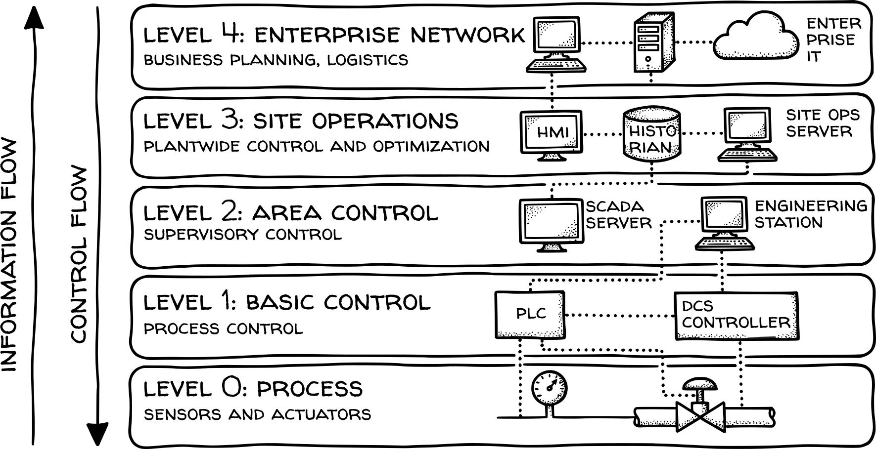
The data characteristics evolves across this hierarchy. At Levels 0-2, data is distinctively high-velocity and high-volume, comprising real-time sensor streams and control signals required for immediate process stability. These high-frequency datasets are typically retained for short periods (hours to weeks) to support troubleshooting and loop tuning, with only downsampled aggregates stored long-term. Moving to Levels 3 and 4, data volume decreases while context and aggregation increase; raw time-series measurements are transformed into production metrics, inventory levels, and financial indicators. The Purdue model relies on a rigid hierarchy where data must traverse multiple layers to reach the enterprise, modern architectures are evolving. Increasingly, flatter data access models such as the Unified Name Space (UNS) (Marcy 2023) are being adopted to break down these silos and facilitate real-time analytics.
While Purdue model provides a useful framework for understanding the hierarchy of engineering data, the engineering data that is useful and available for model development is far more diverse. Below are some examples of engineering data that is useful and available for model development.
Process operational and experimental data
The primary source for data-driven modeling is typically process operational data generated by distributed control systems. This includes high-frequency, structured time-series measurements from sensors, control signals, and batch records. Plant operations increasingly supplement these traditional streams with sensor and IoT data such as vibration analysis and acoustic monitoring for predictive maintenance. Visual data from thermal imaging or drone inspections provides another unstructured but high-value source for specialized monitoring applications. In contrast, experimental data from bench-scale studies and pilot plants offers lower volume but high-value information critical for validation. Closely related to operations is maintenance and asset data, which links process conditions to equipment health through event-based logs and reliability metrics.
Engineering and simulation data
First-principles and hybrid models rely heavily on design and engineering data, including P&IDs, equipment specifications, and geometric models from CAD systems. This physical context is supported by materials and physical properties data, a tabular reference category comprising pure component properties and safety data sheets. When experimental data is scarce, simulation and modeling data from process simulators (Aspen Plus, gPROMS) or CFD tools can serve as high-volume surrogate datasets. Additionally, regulatory and compliance data such as emissions logs and safety reports (HAZOP) imposes strict boundary conditions on model validity and operation.
Business and contextual data
Beyond the battery limit, models increasingly integrate economic and business data to drive optimization based on profitability rather than just yield. This financial context—capital costs, utility pricing, and market data—is often time-varying and strategic. Supply chain and logistics data provides transactional context on raw material quality and inventory levels. Broader environmental context is provided by geospatial and environmental data, including meteorological conditions and site coordinates. Finally, unstructured knowledge resides in literature and knowledge data (research papers, patents) and human and organizational data (operator logs, shift notes), which capture essential “tribal knowledge” but remain difficult to integrate directly into quantitative workflows.
3.4.2 Dimensions of engineering data
Engineering data is defined by several key dimensions (Figure 3.5). Volume refers to the sheer scale of data generated, ranging from gigabytes of daily sensor logs to singular, high-value design documents. Velocity captures the speed of data generation and processing, spanning from millisecond-level real-time control signals to static reference data that remains unchanged for years. Beyond these, data is characterized by variety and veracity. Process data encompasses diverse formats including structured time-series, semi-structured logs, and unstructured images or documents. Veracity refers to data quality and uncertainty; calibrated sensors provide high-fidelity measurements, whereas soft sensors or human inputs introduce significant ambiguity. The value of data is highly context-dependent. A single failure report may hold more strategic insight than terabytes of routine temperature logs. Data lifecycle management is critical, as transient control errors may be discarded immediately while regulatory compliance records must remain accessible for decades. Furthermore, data ownership is often fragmented across proprietary corporate systems, personal records, and public databases, complicating integration efforts due to disparate formats and inconsistent taxonomies.
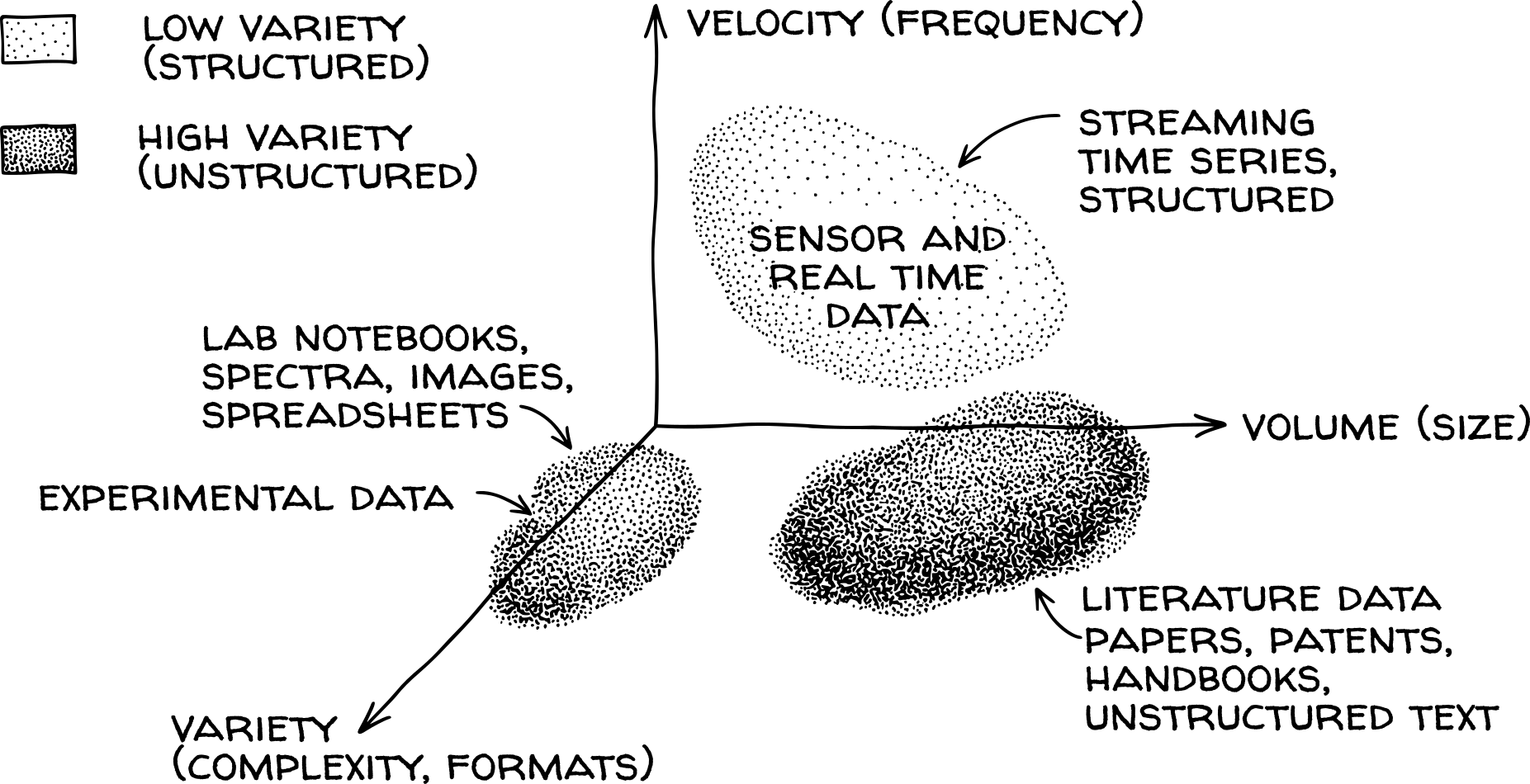
The choice of modeling strategy determines the data requirements. Table 3.2 summarizes the data requirements for different modeling strategies. First-principles models use engineering parameters such as equipment geometry and thermodynamic constants (Level 3). These parameters come from static specifications or laboratory systems. Data-driven models use time-series data from sensors and control loops (Levels 1 and 2). This data provides dense temporal information but often includes noise or compression artifacts that require preprocessing. Hybrid architectures combine these sources. They use fundamental parameters to constrain the model and operational data to calibrate empirical components.
| Model Type | Primary Data Needs | Volume | Quality |
|---|---|---|---|
| First-principles | Fundamental properties, structure | Low | Very High |
| Empirical/Regression | Training/validation sets | Medium | High |
| Data-driven/ML | Historical operating data | Very High | Medium |
| Hybrid | All of the above | High | High |
Modelers rarely receive analysis-ready data. Information exists in separate, incompatible formats. Sensor data typically consists of high-frequency CSV files with unsynchronized timestamps. Experimental results appear in Excel spreadsheets or handwritten laboratory notebooks. Photographs and videos capture equipment conditions or sample appearance. Physical property data often exists as static graph images in literature, which requires digitization. Operational context, such as maintenance events, appears in unstructured PDF shift logs. The modeler must combine these sources programmatically by resampling signals, digitizing graphs, and parsing text to create a unified dataset.
3.5 Terminology for data-driven modeling
Developing a robust data-driven model begins with a structured understanding of the available data. To facilitate further discussion, we define the terminology used to describe data in data-driven modeling. Process variables are categorized by their role, measurability, temporal behavior, and usage in modeling.
By role in process
- Inputs are independent variables that drive the process. These include:
- Manipulated variables: inputs that can be actively controlled (e.g., valve positions, pump speeds)
- Disturbances: unmeasured or uncontrolled inputs that affect the process (e.g., ambient temperature, feed composition variations)
- Outputs are dependent responses that result from the process (e.g., product quality, reactor temperature, conversion rate).
- State variables are internal process conditions that fully describe the system state at any given time (e.g., reactant concentrations, internal temperatures).
- Parameters are system constants that characterize the process but do not change during normal operation (e.g., heat transfer coefficients, reaction rate constants, equipment dimensions).
By measurability
- Measured variables are variables that are directly observed through sensors or instrumentation (e.g., temperature sensors, flow meters, pressure transducers).
- Inferred/Estimated variables are variables that are calculated or estimated from other measurements, often using soft sensors or estimators (e.g., product composition inferred from temperature and pressure).
- Unmeasured variables are variables that are neither directly measured nor inferred, but may still influence the process (e.g., catalyst activity, fouling factors).
By temporal behavior
- Static variables are time-invariant and remain constant during the period of interest (e.g., equipment specifications, fixed setpoints).
- Dynamic variables are time-varying and change over time in response to process conditions (e.g., temperature profiles, concentration trajectories).
- Stochastic variables exhibit random behavior and contain noise or uncertainty (e.g., measurement noise, random disturbances).
By data usage
- Training data is the dataset used to fit or train the model parameters.
- Validation data is a held-out dataset used during model development to tune hyperparameters and prevent overfitting. Hyperparameters are parameters that are not learned from the data, but are set by the modeler before training.
- Test data is a final held-out dataset used to evaluate model performance on unseen data.
- Inference/Production data is real-time or new data on which the trained model makes predictions during deployment.
3.5.1 Data characteristics
Beyond variable classification, data exhibits structural properties that affect modeling:
- Drift refers to changes in data properties over time. Sensor drift is gradual loss of calibration. Concept drift occurs when the underlying process relationship changes, for example, change in reaction rate constant due to catalyst deactivation. Both require periodic model retraining or adaptive methods.
- Autocorrelation is the correlation of a signal with its own past values. Process measurements sampled at high frequency are strongly autocorrelated, meaning successive samples are not independent. This inflates apparent dataset size and violates assumptions of standard regression models.
- Collinearity describes strong linear relationships between input variables. Many process variables move together, for example, reactor temperature and pressure. Collinearity destabilizes regression coefficients and complicates interpretation.
- Bias is a systematic offset between a measurement and the true value. Measurement bias arises from sensor installation, calibration error, or environmental effects. Selection bias occurs when training data is not representative of the full operating envelope, for example, training only on normal operation while ignoring upsets.
3.5.2 Machine learning terminology in process context
Standard machine learning terminology requires reinterpretation for process data:
- Features are the input variables used by the model. In process contexts, features carry physical units and constraints. A temperature feature cannot be negative Kelvin; a composition must remain between 0 and 100%. Feature engineering must respect these bounds.
- Overfitting occurs when a model fits training data too closely and fails to generalize. In process models, overfitting often manifests as predictions that violate conservation laws or thermodynamic limits outside the training range.
- Cross-validation is a technique for estimating model performance by partitioning data. Standard k-fold cross-validation assumes independent samples, which is violated by autocorrelated time-series. Time-series cross-validation requires forward-chaining splits that respect temporal order.
3.6 Data quality issues
Data-driven modeling begins with data, however, the data a modeler receives is rarely clean or well-organized. The data sources described in Section 3.4 each bring characteristic quality problems. Before any model can be trained, this raw data must be understood and conditioned. The first step is recognizing what can go wrong.
Operational data from DCS and historians is most susceptible to sensor faults, multi-rate sampling, and timestamp drift. Lab and experimental data suffers from missing values that are not random and subject to transcription errors when entered manually. Engineering and simulation data introduces model-reality mismatch, version control issues. Business and contextual data such as batch IDs, work orders, product codes may carry labeling and metadata errors that silently propagate into any analysis that joins across systems. Recognizing which quality issues are likely for each data source helps focus diagnostic effort where it matters most.
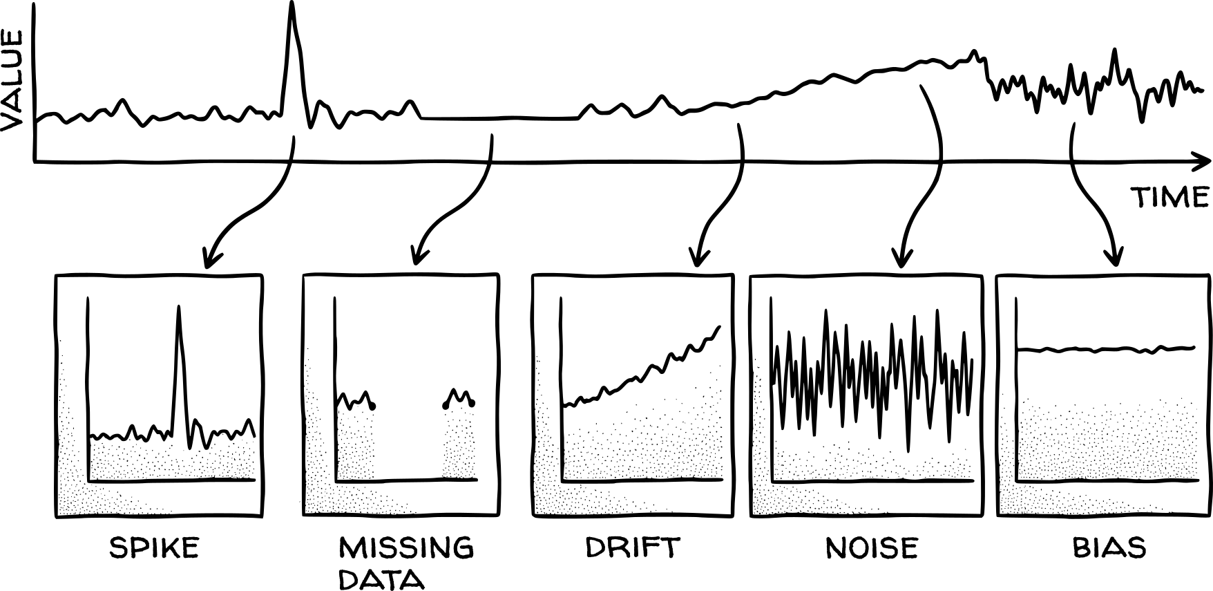
Industrial time-series data is rarely clean. Sensors degrade, communication links fail, and instrumentation introduces artifacts that corrupt the recorded signal. Figure 3.6 illustrates five commonly encountered anomalies. A spike is a transient excursion far from the baseline, often caused by electrical interference, valve hammering, or sample injection artifacts. Missing data appears as gaps where no values are recorded, whether from sensor outage, communication failure, or deliberate exclusion during maintenance. Drift is a slow monotonic shift in the signal level over time, typically from sensor degradation, fouling, or calibration loss. Noise manifests as rapid random fluctuations superimposed on the true signal, arising from electrical pickup, turbulence, or quantization effects. Bias is a constant offset between the measured value and the true value, caused by calibration error, installation effects, or systematic measurement distortion. These patterns frequently coexist in the same time series, and a single root cause can produce several of them simultaneously.
3.7 Data preprocessing
Recognizing data quality issues is only the first step. Before any modeling can begin, the raw data must be conditioned. Gaps must be filled, outliers handled, time series aligned, and operating regimes identified. This section provides a brief overview of common preprocessing steps. A full treatment of data cleaning and feature engineering is beyond the scope of this text. Several excellent resources exist for those seeking deeper coverage. Bagajewicz, Chmielewski, and Tanth (2010) covers the design and operation of process data systems, including sensor networks, data validation, and the software infrastructure that supports plant-wide data management. Kuhn and Johnson (2021) addresses feature engineering and variable selection in the context of predictive modeling, with examples that apply across domains including process systems. Narasimhan and Jordache (2000) focuses specifically on data reconciliation and gross error detection, presenting the mathematical framework for adjusting measured values to satisfy mass and energy balances while identifying faulty sensors.
The raw data extracted from a process historian is rarely suitable for direct use in modeling. Historians such as AVEVA Historian (www.aveva.com n.d.), Siemens SIMATIC PCS 7 (siemens.com n.d.), and dataPARC (www.dataparc.com n.d.) typically store data using exception-based compression. In this method, a new value is recorded only when the signal changes by more than a configured deadband. This reduces storage but produces irregular time stamps and creates the illusion of flat periods that may or may not reflect true process behavior. The first preprocessing task is to understand how the historian stores and compresses data, and to extract the raw event stream rather than pre-interpolated values when possible.
Most modeling algorithms expect data to be at equal time intervals (constant \(\Delta t\)). Reconstruction converts the irregular historian events into a regular series at a chosen sample interval. The choice of interval depends on the fastest dynamics of interest. For thermal systems that typically have a slow response time, sampling every minute may be adequate, but a fast response signal like a pressure signal may require sampling every second. Two common reconstruction methods are zero-order hold and linear interpolation. Zero-order hold forward-fills the last known value until the next event, which is appropriate for setpoints, valve states, and other discrete signals. Linear interpolation connects successive events with a straight line, which suits continuous physical variables but can create false trends between events that were actually flat. Documentary-style historian exports often apply interpolation before export, so the modeler may need to request raw event data to control the reconstruction method.
Industrial data comes from sources with different sample rates. Regulatory tags (temperature, pressure, flow) may update every second, while composition analyzers report every few minutes and lab samples arrive once per shift. Aligning these sources onto a common time grid requires care.
A simple approach would be to repeat the slow variable at every fast time step. However, this can introduce future information if the alignment is not strictly causal. For example, using a lab value recorded at 10:00 to label all rows from 08:00 onward leaks the future into the training set. A better approach would be to lag the slow variable so that each row uses only information available at that time. For composition analyzers with known sample delays, the delay should be modeled explicitly.
Many models assume the process operates near a steady state where the mean and variance of key variables are approximately constant. Startups, shutdowns, grade transitions, and upset recoveries violate this assumption and can confuse models trained on steady-state data or near steady-state data. Steady-state detection identifies periods where the process is stable enough for model training or validation. A common technique is to calculate the rolling variance of key variables over a window; if the variance remains below a threshold for a specified duration, that period is flagged as steady. Another technique is to use the R-statistic defined as (\(R = {s^2_{\text{long}}}/{s^2_{\text{short}}}\)), which is the ratio of the variance at two different window sizes. A value of \(R \approx 1\) suggests stationarity. A value of \(R > 1\) indicates a drifting mean, while \(R < 1\) indicates a recent transient or disturbance. Either deviation from unity flags the period as non-steady. Excluding non-steady periods from training improves model accuracy but requires careful logging so the modeler knows what fraction of the data was used.
Outliers are data points that deviate markedly from the expected range. In process data, they arise from transient physical events (valve slam, pump cavitation), instrumentation artifacts (electrical interference, sensor saturation), or data entry errors. Simple univariate tests such as values outside three standard deviations or outside physical limits catch the most obvious cases. Multivariate methods like principal component analysis (PCA) or clustering can detect points that are unusual in combination even if each variable individually looks normal. Once detected, outliers can be removed, replaced with interpolated values, or flagged and retained for separate analysis. The choice depends on whether the outlier represents a real event worth studying or a measurement error with no process meaning. Logging the detection rule and the number of points affected is a necessary part of any preprocessing audit trail.
No preprocessing pipeline should be trusted without validation. The simplest check is visual. Plot the raw and processed series together to verify that the transformation is sensible. Mass and energy balances, when available, provide a physics-based sanity check. If the processed data fails to close a balance that the raw data closes (or vice versa), something is wrong. Comparing model performance on data processed with different methods (e.g., zero-order hold vs. linear interpolation) can reveal sensitivity to preprocessing choices. Finally, the preprocessing pipeline should be version-controlled and documented so that results are reproducible and so that future analysts understand what was done and why.
3.8 Data driven modeling workflow
A data-driven modeling workflow for process systems proceeds through eight distinct phases, as illustrated in Figure 3.7. Each phase has specific inputs, outputs, and failure modes.
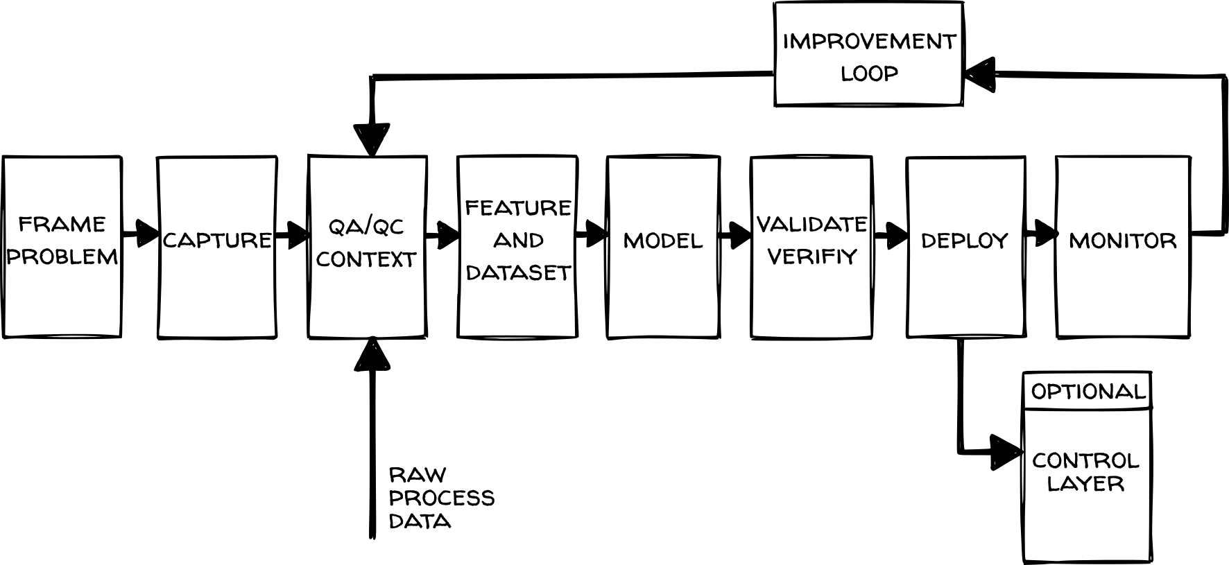
The process begins with problem framing, which establishes the scope before any data is collected. The modeler defines the objective, the target variable and its prediction horizon, the key performance indicators that determine success, and the deployment context. Data collection follows, identifying and retrieving relevant signals from available sources. Process data typically comes from variety of sources including sensors, analyzers, and distributed control systems, laboratory assays, operator logs, and maintenance records. Context tags indicating operating mode, product grade, or campaign identity are essential for segmenting the data appropriately. Data QA/QC and contextualization converts raw signals into analysis-ready form. This phase includes tag mapping, unit verification, timestamp alignment across systems, and identification of bad data such as stuck values, dropouts, or sensor drift. Proper segmentation is necessary to prevent the model from training on mixed regimes. Feature and dataset construction transforms the cleaned data into model inputs. Here, if required, resampling is performed to align signals sampled at different rates. The dataset is then split into training, validation, and test subsets using appropriate strategies.
Model development is largely governed by the problem framing and feature engineering phases. As Occam’s razor suggests, the simplest model that meets the performance requirements is preferred. Validation and verification tests the candidate models under realistic conditions. Both time-based and unit-based splits are used to prevent data leakage. The models are often evaluated using metrics such as mean absolute error, root mean squared error, and R-squared and backtested on historical data. Deployment integrates the validated model into the production environment.
Monitoring and governance tracks model and data health after deployment. Model performance monitors compare predictions to actuals as ground truth becomes available. If any discrepancy is observed, the improvement loop is triggered. This loop may involve retraining the model, updating the QA rules, or refining the feature engineering. For control and optimization use cases, like a model predictive controller (MPC), a separate layer may be used to deploy the model and use its predictions.